从 GCM 生成样本#
图形因果模型 (GCM) 描述了建模变量的数据生成过程。因此,在拟合 GCM 后,我们还可以从中生成全新的样本,因此可以将其视为基于底层模型生成合成数据的生成器。生成新样本通常可以通过以下步骤完成:按拓扑顺序排序节点,从根节点随机采样,然后通过使用随机采样的噪声评估下游因果机制将数据传播到图中。dowhy.gcm 软件包提供了一个简单的辅助函数来自动完成此操作,从而提供了一个简单的 API 来从 GCM 抽取样本。
让我们看看下面的例子
>>> import numpy as np, pandas as pd
>>>
>>> X = np.random.normal(loc=0, scale=1, size=1000)
>>> Y = 2 * X + np.random.normal(loc=0, scale=1, size=1000)
>>> Z = 3 * Y + np.random.normal(loc=0, scale=1, size=1000)
>>> data = pd.DataFrame(data=dict(X=X, Y=Y, Z=Z))
>>> data.head()
          X         Y          Z
0  0.690159  0.619753   1.447241
1 -0.371759 -0.091857  -0.102173
2 -1.555987 -3.103839 -10.888229
3 -1.540165 -3.196612  -9.028178
4  1.218309  3.867429  12.394407
现在,我们基于定义的因果图和加性噪声模型假设,学习了变量的生成模型。要从这个模型中生成新样本,我们现在只需调用
>>> import networkx as nx
>>> import dowhy.gcm as gcm
>>>
>>> causal_model = gcm.StructuralCausalModel(nx.DiGraph([('X', 'Y'), ('Y', 'Z')]))
>>> gcm.auto.assign_causal_mechanisms(causal_model, data) # Automatically assigns additive noise models to non-root nodes
>>> gcm.fit(causal_model, data)
现在,我们基于定义的因果图和加性噪声模型假设,学习了变量的生成模型。要从这个模型中生成新样本,我们现在只需调用
>>> generated_data = gcm.draw_samples(causal_model, num_samples=1000)
>>> generated_data.head()
          X         Y          Z
0 -0.322038 -0.693841  -2.319015
1 -0.526893 -2.058297  -6.935897
2 -1.591554 -4.199653 -12.588653
3 -0.817718 -1.125724  -3.013189
4  0.520793 -0.081344   0.987426
如果我们的建模假设是正确的,生成的数据现在应该类似于观测到的数据分布,也就是说,生成的样本对应于我们开始时为示例数据定义的联合分布。确保这一点的一种方法是估计观测分布和生成分布之间的 KL 散度。为此,我们可以利用评估模块
>>> print(gcm.evaluate_causal_model(causal_model, data, evaluate_causal_mechanisms=False, evaluate_invertibility_assumptions=False))
Evaluated and the overall average KL divergence between generated and observed distribution and graph structure. The results are as follows:
==== Evaluation of Generated Distribution ====
The overall average KL divergence between the generated and observed distribution is 0.014769479715506385
The estimated KL divergence indicates an overall very good representation of the data distribution.
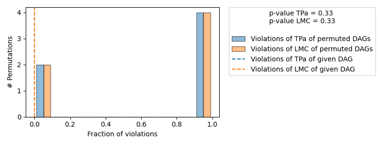
==== Evaluation of the Causal Graph Structure ====
+-------------------------------------------------------------------------------------------------------+
| Falsification Summary |
+-------------------------------------------------------------------------------------------------------+
| The given DAG is not informative because 2 / 6 of the permutations lie in the Markov |
| equivalence class of the given DAG (p-value: 0.33). |
| The given DAG violates 0/1 LMCs and is better than 66.7% of the permuted DAGs (p-value: 0.33). |
| Based on the provided significance level (0.2) and because the DAG is not informative, |
| we do not reject the DAG. |
+-------------------------------------------------------------------------------------------------------+
==== NOTE ====
Always double check the made model assumptions with respect to the graph structure and choice of causal mechanisms.
All these evaluations give some insight into the goodness of the causal model, but should not be overinterpreted, since some causal relationships can be intrinsically hard to model. Furthermore, many algorithms are fairly robust against misspecifications or poor performances of causal mechanisms.
这证实了生成的分布与观测分布接近。
注意
虽然评估也为我们提供了有关因果图结构的见解,但我们无法确认图结构,只能在我们发现观测结构依赖关系与图表示之间存在不一致时驳斥它。在我们的案例中,我们不驳斥 DAG,但还有其他等价的 DAG 也不会被驳斥。要理解这一点,请考虑上面的示例——X→Y→Z 和 X←Y←Z 将生成相同的观测分布(因为它们编码相同的条件分布),但只有 X→Y→Z 会生成正确的干预分布(例如,当干预 Y 时)。
下一节提供了有关评估方法的更多详细信息。