评估 GCM#
对图形因果模型 (GCM) 进行建模需要各种假设和模型选择,所有这些都会影响模型的性能和准确性。所需的假设示例包括
图结构: 正确指定变量之间的因果方向至关重要。例如,说下雨导致街道湿润是合乎逻辑的,而声称街道湿润导致下雨则没有意义。如果这些关系建模不正确,由此产生的因果陈述将具有误导性。然而,需要注意的是,虽然这个例子非常直观,但模型通常对错误指定表现出一定程度的鲁棒性。特别是在较大的图中,错误指定的影响往往不太严重。此外,错误指定的严重程度可能有所不同;例如,定义错误的因果方向通常比将过多的(上游)节点包含为某个节点的潜在父节点更成问题。
由于因果图结构定义了关于变量之间(条件)独立性的假设,因此可以证伪给定的图结构。例如,在链 X→Y→Z 中,我们知道在给定 Y 的情况下,X 和 Z 必须相互独立。如果情况并非如此,则我们有一些证据表明给定的图是错误的。然而,另一方面,如果没有更强的假设,我们无法确认图的正确性。沿用链示例,如果我们翻转两条边,条件独立性陈述(在给定 Y 的情况下,X 独立于 Z)仍然成立。
因果机制假设: 为了对因果数据生成过程进行建模,我们使用形式为 \(X_i = f_i(PA_i, N_i)\) 的因果机制表示每个节点,其中 \(N_i\) 表示未观察到的噪声,\(PA_i\) 表示 \(X_i\) 的因果父节点。在这种情况下,我们需要对函数 \(f_i\) 的形式进行额外假设。例如,对于连续变量,通常使用形式为 \(X_i = f_i(PA_i) + N_i\) 的加性噪声模型对 \(f_i\) 进行建模。然而,如果真实关系不同(例如,乘性关系),这种表示可能不准确。因此,因果机制的类型是另一个可能影响结果的因素。然而,总的来说,在连续情况下,加性噪声模型假设在实践中往往相对鲁棒,不易受到违反的影响。
模型选择: 前两点仅侧重于准确表示变量之间的因果关系。现在,模型选择过程增加了一个额外的层面。以加性噪声模型 \(X_i = f_i(PA_i) + N_i\) 为例,模型选择的挑战在于确定 \(f_i\) 的最优模型。理想情况下,这将是使均方误差最小化的模型。
考虑到影响 GCM 性能的多种因素,每种因素都有自己的指标和挑战,dowhy.gcm 提供了一个模块,旨在评估拟合的 GCM 并提供不同评估指标的概览。此外,如果使用自动分配,我们可以获得选择过程中评估的模型和性能的概览。
自动分配摘要#
如果关于因果关系的先验知识可用,则始终建议使用该知识相应地建模因果机制。然而,如果缺乏足够的洞察力,GCM 的自动分配功能可以帮助根据给定数据自动为每个节点选择合适的因果机制。自动分配执行两项任务:1) 选择合适的因果机制,2) 从小型模型库中选择性能最佳的模型。
使用自动分配功能时,我们可以获得有关模型选择过程的额外洞察力,例如考虑的因果机制类型以及评估的模型及其性能。为了说明这一点,再次考虑链结构示例 X→Y→Z
>>> import numpy as np, pandas as pd
>>> import networkx as nx
>>> import dowhy.gcm as gcm
>>>
>>> X = np.random.normal(loc=0, scale=1, size=1000)
>>> Y = 2 * X + np.random.normal(loc=0, scale=1, size=1000)
>>> Z = 3 * Y + np.random.normal(loc=0, scale=1, size=1000)
>>> data = pd.DataFrame(data=dict(X=X, Y=Y, Z=Z))
>>>
>>> causal_model = gcm.StructuralCausalModel(nx.DiGraph([('X', 'Y'), ('Y', 'Z')]))
>>> summary_auto_assignment = gcm.auto.assign_causal_mechanisms(causal_model, data)
>>> print(summary_auto_assignment)
When using this auto assignment function, the given data is used to automatically assign a causal mechanism to each node. Note that causal mechanisms can also be customized and assigned manually.
The following types of causal mechanisms are considered for the automatic selection:

If root node:
An empirical distribution, i.e., the distribution is represented by randomly sampling from the provided data. This provides a flexible and non-parametric way to model the marginal distribution and is valid for all types of data modalities.

If non-root node and the data is continuous:
Additive Noise Models (ANM) of the form X_i = f(PA_i) + N_i, where PA_i are the parents of X_i and the unobserved noise N_i is assumed to be independent of PA_i.To select the best model for f, different regression models are evaluated and the model with the smallest mean squared error is selected.Note that minimizing the mean squared error here is equivalent to selecting the best choice of an ANM.

If non-root node and the data is discrete:
Discrete Additive Noise Models have almost the same definition as non-discrete ANMs, but come with an additional constraint for f to only return discrete values.
Note that 'discrete' here refers to numerical values with an order. If the data is categorical, consider representing them as strings to ensure proper model selection.

If non-root node and the data is categorical:
A functional causal model based on a classifier, i.e., X_i = f(PA_i, N_i).
Here, N_i follows a uniform distribution on [0, 1] and is used to randomly sample a class (category) using the conditional probability distribution produced by a classification model.Here, different model classes are evaluated using the (negative) F1 score and the best performing model class is selected.

In total, 3 nodes were analyzed:

--- Node: X
Node X is a root node. Therefore, assigning 'Empirical Distribution' to the node representing the marginal distribution.

--- Node: Y
Node Y is a non-root node with continuous data. Assigning 'AdditiveNoiseModel using LinearRegression' to the node.
This represents the causal relationship as Y := f(X) + N.
For the model selection, the following models were evaluated on the mean squared error (MSE) metric:
LinearRegression: 0.9978767184153945
Pipeline(steps=[('polynomialfeatures', PolynomialFeatures(include_bias=False)),
                ('linearregression', LinearRegression)]): 1.00448207264867
HistGradientBoostingRegressor: 1.1386270868995179

--- Node: Z
Node Z is a non-root node with continuous data. Assigning 'AdditiveNoiseModel using LinearRegression' to the node.
This represents the causal relationship as Z := f(Y) + N.
For the model selection, the following models were evaluated on the mean squared error (MSE) metric:
LinearRegression: 1.0240822102491627
Pipeline(steps=[('polynomialfeatures', PolynomialFeatures(include_bias=False)),
                ('linearregression', LinearRegression)]): 1.02567150836141
HistGradientBoostingRegressor: 1.358002751994007

===Note===
Note, based on the selected auto assignment quality, the set of evaluated models changes.
For more insights toward the quality of the fitted graphical causal model, consider using the evaluate_causal_model function after fitting the causal mechanisms.
在此场景中,经验分布被分配给根节点 X,而节点 Y 和 Z 则使用加性噪声模型(有关因果机制类型的更多详细信息,请参阅图形因果模型的类型)。在这两种情况下,线性回归模型在最小化均方误差方面表现最佳。评估的模型及其性能列表也可用。由于我们使用了自动分配的默认参数,因此只评估了一个小型模型库。然而,我们也可以调整分配质量以扩展到更多模型。
为每个节点分配因果机制后,后续步骤涉及将这些机制拟合到数据中
>>> gcm.fit(causal_model, data)
评估拟合的 GCM#
因果模型已拟合,可用于解决不同的因果问题。然而,我们可能首先有兴趣了解因果模型的性能,即我们可能想知道
我的因果机制表现如何?
加性噪声模型假设对我的数据是否有效?
GCM 是否捕获了观测数据的联合分布?
我的因果图结构是否与数据兼容?
为此,我们可以使用因果模型评估功能,该功能为我们提供了有关整体模型性能以及我们的假设是否成立的一些见解
>>> summary_evaluation = gcm.evaluate_causal_model(causal_model, data, compare_mechanism_baselines=True)
>>> print(summary_evaluation)
Evaluated the performance of the causal mechanisms and the invertibility assumption of the causal mechanisms and the overall average KL divergence between generated and observed distribution and the graph structure. The results are as follows:
==== Evaluation of Causal Mechanisms ====
The used evaluation metrics are:
- KL divergence (only for root-nodes): Evaluates the divergence between the generated and the observed distribution.
- Mean Squared Error (MSE): Evaluates the average squared differences between the observed values and the conditional expectation of the causal mechanisms.
- Normalized MSE (NMSE): The MSE normalized by the standard deviation for better comparison.
- R2 coefficient: Indicates how much variance is explained by the conditional expectations of the mechanisms. Note, however, that this can be misleading for nonlinear relationships.
- F1 score (only for categorical non-root nodes): The harmonic mean of the precision and recall indicating the goodness of the underlying classifier model.
- (normalized) Continuous Ranked Probability Score (CRPS): The CRPS generalizes the Mean Absolute Percentage Error to probabilistic predictions. This gives insights into the accuracy and calibration of the causal mechanisms.
NOTE: Every metric focuses on different aspects and they might not consistently indicate a good or bad performance.
We will mostly utilize the CRPS for comparing and interpreting the performance of the mechanisms, since this captures the most important properties for the causal model.
--- Node X
- The KL divergence between generated and observed distribution is 0.04082997872632467.
The estimated KL divergence indicates an overall very good representation of the data distribution.
--- Node Y
- The MSE is 0.9295878353315775.
- The NMSE is 0.44191515264388137.
- The R2 coefficient is 0.8038281270395207.
- The normalized CRPS is 0.25235753447337383.
The estimated CRPS indicates a good model performance.
The mechanism is better or equally good than all 7 baseline mechanisms.
--- Node Z
- The MSE is 0.9485970223031653.
- The NMSE is 0.14749131486369138.
- The R2 coefficient is 0.9781306148527433.
- The normalized CRPS is 0.08386782069483441.
The estimated CRPS indicates a very good model performance.
The mechanism is better or equally good than all 7 baseline mechanisms.
==== Evaluation of Invertible Functional Causal Model Assumption ====
--- The model assumption for node Y is not rejected with a p-value of 1.0 (after potential adjustment) and a significance level of 0.05.
This implies that the model assumption might be valid.
--- The model assumption for node Z is not rejected with a p-value of 1.0 (after potential adjustment) and a significance level of 0.05.
This implies that the model assumption might be valid.
Note that these results are based on statistical independence tests, and the fact that the assumption was not rejected does not necessarily imply that it is correct. There is just no evidence against it.
==== Evaluation of Generated Distribution ====
The overall average KL divergence between the generated and observed distribution is 0.015438550831663324
The estimated KL divergence indicates an overall very good representation of the data distribution.
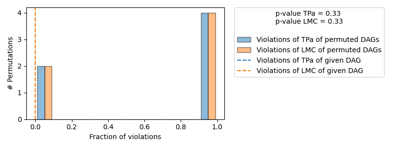
==== Evaluation of the Causal Graph Structure ====
+-------------------------------------------------------------------------------------------------------+
| Falsification Summary |
+-------------------------------------------------------------------------------------------------------+
| The given DAG is not informative because 2 / 6 of the permutations lie in the Markov |
| equivalence class of the given DAG (p-value: 0.33). |
| The given DAG violates 0/1 LMCs and is better than 66.7% of the permuted DAGs (p-value: 0.33). |
| Based on the provided significance level (0.2) and because the DAG is not informative, |
| we do not reject the DAG. |
+-------------------------------------------------------------------------------------------------------+
==== NOTE ====
Always double check the made model assumptions with respect to the graph structure and choice of causal mechanisms.
All these evaluations give some insight into the goodness of the causal model, but should not be overinterpreted, since some causal relationships can be intrinsically hard to model. Furthermore, many algorithms are fairly robust against misspecifications or poor performances of causal mechanisms.
正如我们所见,我们可以获得不同评估的详细概览
因果机制评估: 根据模型性能评估因果机制。对于非根节点,最重要的度量标准是(归一化)连续排序概率得分 (CRPS),它提供了关于机制准确性及其作为概率模型的校准的洞察。它还列出了其他指标,例如均方误差 (MSE)、按方差归一化的 MSE(表示为 NMSE)、R2 系数,以及对于分类变量的 F1 分数。如果节点是根节点,则测量生成数据分布和观测数据分布之间的 KL 散度。
可选地,我们可以将 compare_mechanism_baselines 参数设置为 True,以便将机制与一些基线模型进行比较。这让我们更好地了解机制与其他模型相比的性能。但是请注意,这对于较大的图可能需要相当长的时间。
可逆函数因果模型假设评估: 如果因果机制是可逆函数因果模型,我们可以验证该假设是否成立。请注意,这里的可逆函数是指相对于噪声而言,即加性噪声模型 \(X_i = f_i(PA_i) + N_i\) 以及更一般的后非线性模型 \(X_i = g_i(f_i(PA_i) + N_i)\)(其中 \(g_i\) 是可逆的)就是此类机制的示例。在这种情况下,基于观测估计的噪声应独立于输入。
生成分布评估: 由于 GCM 能够从学习到的分布生成新的样本,我们可以评估生成的(联合)分布是否与观测分布一致。在这里,差异应尽可能小。为了使 KL 散度估计对于潜在的大型图可行,通过计算每个节点生成分布和观测边缘分布之间的 KL 散度的平均值来近似。
因果图结构评估: 如上所述,图结构应表示观测数据中的(条件)独立性(假设忠实性)。这可以用来通过运行不同的独立性检验,了解给定的图是否违反了基于数据的(不)独立性结构。为此,使用了一种算法来检查图是否可以被拒绝,以及是否能够从这种独立性检验中获得有益的见解。
请注意,所有这些评估方法仅提供对给定 GCM 的一些见解,但不能完全确认学习模型的正确性。有关指标和评估方法的更多详细信息,请参阅相应方法的文档字符串。