使用 DoWhy 和 EconML 计算条件平均治疗效果 (CATE)#
这是一项实验性功能,我们在其中使用 DoWhy 中的 EconML 方法。使用 EconML 可以通过不同方法进行 CATE 估计。
DoWhy 中因果推断的所有四个步骤保持不变:建模、识别、估计和反驳。主要区别在于我们现在在估计步骤中调用 econml 方法。还有一个使用线性回归的简单示例,以帮助理解 CATE 估计器背后的直觉。
所有数据集均使用线性结构方程生成。
[1]:
%load_ext autoreload
%autoreload 2
[2]:
import numpy as np
import pandas as pd
import logging

import dowhy
from dowhy import CausalModel
import dowhy.datasets

import econml
import warnings
warnings.filterwarnings('ignore')

BETA = 10
[3]:
data = dowhy.datasets.linear_dataset(BETA, num_common_causes=4, num_samples=10000,
                                    num_instruments=2, num_effect_modifiers=2,
                                     num_treatments=1,
                                    treatment_is_binary=False,
                                    num_discrete_common_causes=2,
                                    num_discrete_effect_modifiers=0,
                                    one_hot_encode=False)
df=data['df']
print(df.head())
print("True causal estimate is", data["ate"])
         X0        X1   Z0        Z1        W0        W1 W2 W3         v0  \
0 -0.520835  0.756229  0.0  0.547725 -0.348991 -0.917974  0  3  14.006824
1 -1.560984  0.546710  0.0  0.474327 -0.652985 -1.886253  0  2   5.116915
2 -0.631737  0.866077  0.0  0.993189 -0.317968  0.702546  2  2  20.962792
3 -1.471904  0.208802  1.0  0.543871 -1.858522 -2.549787  0  2   9.131259
4 -2.163623  1.074842  1.0  0.522107 -0.281958  0.102664  1  2  24.442475

            y
0  181.573850
1   56.379803
2  274.811687
3   80.831273
4  301.137661
True causal estimate is 11.573149205663968
[4]:
model = CausalModel(data=data["df"],
                    treatment=data["treatment_name"], outcome=data["outcome_name"],
                    graph=data["gml_graph"])
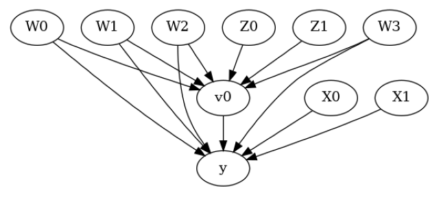
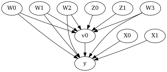
[5]:
model.view_model()
from IPython.display import Image, display
display(Image(filename="causal_model.png"))
[6]:
identified_estimand= model.identify_effect(proceed_when_unidentifiable=True)
print(identified_estimand)
Estimand type: EstimandType.NONPARAMETRIC_ATE

### Estimand : 1
Estimand name: backdoor
Estimand expression:
  d
─────(E[y|W3,W2,W1,W0])
d[v₀]
Estimand assumption 1, Unconfoundedness: If U→{v0} and U→y then P(y|v0,W3,W2,W1,W0,U) = P(y|v0,W3,W2,W1,W0)

### Estimand : 2
Estimand name: iv
Estimand expression:
 ⎡                              -1⎤
 ⎢    d        ⎛    d          ⎞  ⎥
E⎢─────────(y)⋅⎜─────────([v₀])⎟  ⎥
 ⎣d[Z₀  Z₁]    ⎝d[Z₀  Z₁]      ⎠  ⎦
Estimand assumption 1, As-if-random: If U→→y then ¬(U →→{Z0,Z1})
Estimand assumption 2, Exclusion: If we remove {Z0,Z1}→{v0}, then ¬({Z0,Z1}→y)

### Estimand : 3
Estimand name: frontdoor
No such variable(s) found!
线性模型#
首先,让我们使用线性模型建立一些估计 CATE 的直觉。效应调节器(导致异质治疗效果)可以建模为与治疗的交互项。因此,它们的值调节治疗的效果。
下面是治疗从 0 变为 1 的估计效果。
[7]:
linear_estimate = model.estimate_effect(identified_estimand,
                                        method_name="backdoor.linear_regression",
                                       control_value=0,
                                       treatment_value=1)
print(linear_estimate)
*** Causal Estimate ***

## Identified estimand
Estimand type: EstimandType.NONPARAMETRIC_ATE

### Estimand : 1
Estimand name: backdoor
Estimand expression:
  d
─────(E[y|W3,W2,W1,W0])
d[v₀]
Estimand assumption 1, Unconfoundedness: If U→{v0} and U→y then P(y|v0,W3,W2,W1,W0,U) = P(y|v0,W3,W2,W1,W0)

## Realized estimand
b: y~v0+W3+W2+W1+W0+v0*X0+v0*X1
Target units:

## Estimate
Mean value: 11.573167881816286
### Conditional Estimates
__categorical__X0  __categorical__X1
(-4.375, -1.64]    (-3.165, -0.208]      5.078562
                   (-0.208, 0.387]       8.485901
                   (0.387, 0.892]       10.316470
                   (0.892, 1.479]       12.246467
                   (1.479, 4.369]       15.190344
(-1.64, -1.05]     (-3.165, -0.208]      6.211164
                   (-0.208, 0.387]       9.229992
                   (0.387, 0.892]       11.081200
                   (0.892, 1.479]       13.054074
                   (1.479, 4.369]       16.098330
(-1.05, -0.546]    (-3.165, -0.208]      6.672065
                   (-0.208, 0.387]       9.717292
                   (0.387, 0.892]       11.599016
                   (0.892, 1.479]       13.509362
                   (1.479, 4.369]       16.612933
(-0.546, 0.0363]   (-3.165, -0.208]      6.791592
                   (-0.208, 0.387]      10.133414
                   (0.387, 0.892]       12.047274
                   (0.892, 1.479]       13.993364
                   (1.479, 4.369]       17.081919
(0.0363, 2.709]    (-3.165, -0.208]      7.808295
                   (-0.208, 0.387]      10.903614
                   (0.387, 0.892]       12.788630
                   (0.892, 1.479]       14.663872
                   (1.479, 4.369]       18.027674
dtype: float64
EconML 方法#
现在我们转向 EconML 包中更高级的方法来估计 CATE。
首先,让我们看看双重机器学习估计器。Method_name 对应于我们要使用的类的完全限定名称。对于双重 ML,它是“econml.dml.DML”。
目标单位定义了计算因果估计的单位。这可以是应用于原始数据框的 lambda 函数过滤器、新的 Pandas 数据框,或者对应于三种主要目标单位(“ate”、“att”和“atc”)的字符串。下面我们展示一个 lambda 函数的示例。
Method_params 直接传递给 EconML。有关允许参数的详细信息,请参阅 EconML 文档。
[8]:
from sklearn.preprocessing import PolynomialFeatures
from sklearn.linear_model import LassoCV
from sklearn.ensemble import GradientBoostingRegressor
dml_estimate = model.estimate_effect(identified_estimand, method_name="backdoor.econml.dml.DML",
                                     control_value = 0,
                                     treatment_value = 1,
                                 target_units = lambda df: df["X0"]>1,  # condition used for CATE
                                 confidence_intervals=False,
                                method_params={"init_params":{'model_y':GradientBoostingRegressor(),
                                                              'model_t': GradientBoostingRegressor(),
                                                              "model_final":LassoCV(fit_intercept=False),
                                                              'featurizer':PolynomialFeatures(degree=1, include_bias=False)},
                                               "fit_params":{}})
print(dml_estimate)
*** Causal Estimate ***

## Identified estimand
Estimand type: EstimandType.NONPARAMETRIC_ATE

### Estimand : 1
Estimand name: backdoor
Estimand expression:
  d
─────(E[y|W3,W2,W1,W0])
d[v₀]
Estimand assumption 1, Unconfoundedness: If U→{v0} and U→y then P(y|v0,W3,W2,W1,W0,U) = P(y|v0,W3,W2,W1,W0)

## Realized estimand
b: y~v0+W3+W2+W1+W0 | X0,X1
Target units: Data subset defined by a function

## Estimate
Mean value: 13.416786686392697
Effect estimates: [[20.5674886 ]
 [16.81810804]
 [ 4.41081626]
 [12.7590796 ]
 [18.66045567]
 [18.51674086]
 [17.1438172 ]
 [16.72935127]
 [12.3084639 ]
 [10.89723545]
 [12.2995654 ]
 [15.4393769 ]
 [15.12603867]
 [ 9.92507887]
 [21.45669981]
 [14.24272826]
 [ 5.1408623 ]
 [13.95199732]
 [16.10403499]
 [15.51334418]
 [12.86616718]
 [17.69517585]
 [14.98275821]
 [14.02400959]
 [ 8.04652404]
 [ 7.40925404]
 [11.66325528]
 [16.73155822]
 [11.41878005]
 [14.39183237]
 [ 7.78196165]
 [18.5219238 ]
 [ 5.40617633]
 [17.47738011]
 [13.03976874]
 [21.62362646]
 [12.7727103 ]
 [10.89263293]
 [17.30916227]
 [13.97571332]
 [10.90617174]
 [10.42957745]
 [ 8.22825142]
 [16.43221157]
 [12.23764192]
 [12.68420247]
 [11.39128513]
 [16.09066681]
 [10.02702876]
 [ 7.58134396]
 [12.19220932]
 [10.59733045]
 [13.37447019]
 [13.64565928]
 [19.16869052]
 [11.69113092]
 [17.50618788]
 [19.21822674]
 [13.83940523]
 [14.61733979]
 [11.6829634 ]
 [13.74655525]
 [14.36207116]
 [12.77088996]
 [ 9.01665902]
 [11.30305241]
 [15.89790646]
 [11.78357804]
 [16.56510634]
 [14.5326168 ]
 [ 6.39768296]
 [13.43185146]
 [12.01891169]
 [11.60103112]
 [15.70616691]
 [10.93777069]
 [12.58731849]
 [ 9.65958592]
 [17.27134558]
 [10.11003355]
 [12.69721151]
 [14.08728187]
 [13.07706806]
 [13.16812878]
 [13.81273431]
 [10.85485827]
 [11.22442377]
 [11.26772553]
 [10.91163199]
 [18.91911392]
 [14.16473814]
 [12.43741423]
 [10.90886278]
 [15.94262812]
 [ 7.34136344]
 [13.96326514]
 [19.49004536]
 [13.39017623]
 [11.01312687]
 [12.04871674]
 [ 8.74582241]
 [ 9.18646732]
 [14.41435661]
 [ 7.65377335]
 [12.70753593]
 [ 6.5546823 ]
 [20.89621188]
 [13.6687491 ]
 [12.29115227]
 [ 8.23148509]
 [13.14348103]
 [ 8.59881967]
 [14.45936563]
 [12.93855552]
 [14.96923772]
 [15.20999455]
 [ 9.25666362]
 [15.44556932]
 [16.30677664]
 [ 6.79309506]
 [11.0248835 ]
 [11.38621917]
 [12.40392566]
 [15.15631617]
 [15.47750929]
 [13.09407579]
 [21.09243156]
 [14.20065511]
 [18.44004907]
 [17.46505872]
 [13.12384027]
 [10.80277671]
 [12.90042107]
 [10.60835352]
 [15.78490693]
 [12.61665204]
 [10.55847388]
 [17.02018018]
 [ 8.91050269]
 [16.86815955]
 [17.44050478]
 [ 9.96930217]
 [17.72905667]
 [ 9.60855556]
 [12.93686361]
 [12.69410935]
 [13.12214551]
 [10.4047489 ]
 [13.70034905]
 [16.2873264 ]
 [12.54950062]
 [13.07973091]
 [12.94038306]
 [ 8.55823341]
 [14.97447905]
 [12.30526785]
 [ 9.7865365 ]
 [10.0164226 ]
 [ 8.39509301]
 [13.73544153]
 [ 6.24179927]
 [12.11277178]
 [15.53916016]
 [11.05322366]
 [12.12149138]
 [10.06573177]
 [11.90917829]
 [12.56205525]
 [12.90046028]
 [ 9.62295253]
 [18.13306695]
 [17.18491478]
 [15.42384531]
 [11.79491557]
 [14.98991145]
 [15.03724975]
 [11.26121636]
 [12.67032938]
 [ 8.68729779]
 [ 7.51402856]
 [ 9.75685123]
 [12.60398272]
 [12.99152973]
 [15.09644118]
 [16.60299135]
 [16.09588776]
 [ 3.64772799]
 [12.84148723]
 [18.65626365]
 [14.39374335]
 [13.30649259]
 [13.67661457]
 [10.50907391]
 [ 7.14469413]
 [ 9.56842616]
 [ 9.42719284]
 [19.63900172]
 [12.89246116]
 [ 8.51291399]
 [13.26315487]
 [ 9.42047433]
 [11.55964207]
 [11.37217564]
 [ 7.86415732]
 [16.99067817]
 [ 9.95581975]
 [ 7.62928437]
 [15.67276703]
 [15.23104827]
 [14.74048851]
 [11.4638321 ]
 [14.36781003]
 [18.24133044]
 [14.53730603]
 [ 8.93658313]
 [17.13530402]
 [ 9.63114204]
 [14.82085309]
 [14.30631252]
 [13.27430389]
 [22.7958537 ]
 [14.52528945]
 [12.01047948]
 [17.07857452]
 [12.87676195]
 [13.19365817]
 [11.78923515]
 [13.84325536]
 [15.28329488]
 [14.8810602 ]
 [19.02864126]
 [13.24922779]
 [11.08788091]
 [ 9.14628163]
 [12.45375332]
 [13.11554873]
 [16.94156874]
 [15.2703654 ]
 [15.4388345 ]
 [12.66600935]
 [12.21227572]
 [18.48199464]
 [15.73234323]
 [14.98888595]
 [10.50379867]
 [15.36877202]
 [14.41978644]
 [19.1282748 ]
 [ 8.74649804]
 [18.0238775 ]
 [16.50881595]
 [10.51615594]
 [ 5.16953339]
 [20.92100312]
 [12.17479305]
 [14.34722732]
 [ 9.48866414]
 [ 9.27444633]
 [15.30851141]
 [15.60089383]
 [14.87701042]
 [11.39777685]
 [10.39819466]
 [10.52082995]
 [12.78910962]
 [13.08950908]
 [15.14449594]
 [14.14229255]
 [17.33829309]
 [15.11863113]
 [13.36840657]
 [17.27580312]
 [ 9.63258133]
 [13.81493757]
 [15.31935159]
 [16.65902264]
 [18.30038777]
 [10.05234907]
 [15.99178775]
 [14.50080589]
 [19.2293583 ]
 [15.80951257]
 [10.53998897]
 [12.94333869]
 [ 9.27430062]
 [ 7.90520875]
 [ 5.00443678]
 [ 8.62821179]
 [13.16819391]
 [17.04930048]
 [14.83520756]
 [11.11807073]
 [17.01245274]
 [15.80654   ]
 [13.32692666]
 [12.20093365]
 [14.66867576]
 [11.44647894]
 [19.02857772]
 [15.40038588]
 [11.61615852]
 [12.53974592]
 [ 9.5410054 ]
 [11.46179022]
 [16.09647595]
 [10.29908036]
 [10.36165292]
 [17.80286842]
 [17.03426414]
 [14.28988041]
 [ 5.36218566]
 [17.68735257]
 [14.90463919]
 [12.50118809]
 [13.20463625]
 [13.45133909]
 [19.52980369]
 [16.36723555]
 [17.95656214]
 [ 9.07603694]
 [12.99942557]
 [ 7.58217009]
 [12.25094009]
 [20.62468395]
 [15.53609165]
 [15.05133301]
 [13.82908115]
 [14.40748572]
 [11.60776728]
 [13.26077053]
 [ 7.29519633]
 [14.72728296]
 [13.18829522]
 [22.35169842]
 [11.88613095]
 [11.89403583]
 [13.33237917]
 [18.13117447]
 [16.21136452]
 [ 9.46587805]
 [15.05493252]
 [13.11146559]
 [12.94026322]
 [16.74566772]
 [23.87810341]
 [11.38879393]
 [14.16939295]
 [14.46740696]
 [17.20850582]
 [14.87149497]
 [ 9.71447662]
 [ 7.90234328]
 [16.45053096]
 [11.76390866]
 [16.19268945]
 [ 9.99966499]
 [13.66432805]
 [17.05656237]
 [13.16772128]
 [15.21632243]
 [12.74924754]
 [16.00549041]
 [18.74638992]
 [ 8.81325287]
 [20.21752126]
 [14.41172835]
 [11.44879343]
 [13.86334141]
 [16.00583361]
 [ 6.66165918]
 [12.96753674]
 [ 9.60090159]
 [13.28635303]
 [18.4905823 ]
 [ 9.24040548]
 [ 8.27216878]
 [12.17418539]
 [ 6.78689615]
 [13.10914365]
 [ 9.09830979]
 [15.22533319]
 [18.44379055]
 [ 9.53270009]
 [11.06633756]
 [20.46065545]
 [19.78971092]
 [13.14965442]
 [17.03035734]
 [15.86081423]
 [10.07036957]
 [24.56620577]
 [19.94939981]
 [14.09161592]
 [14.38762808]
 [19.65759238]
 [19.37197678]
 [12.76002652]
 [17.86634742]]
[9]:
print("True causal estimate is", data["ate"])
True causal estimate is 11.573149205663968
[10]:
dml_estimate = model.estimate_effect(identified_estimand, method_name="backdoor.econml.dml.DML",
                                     control_value = 0,
                                     treatment_value = 1,
                                 target_units = 1,  # condition used for CATE
                                 confidence_intervals=False,
                                method_params={"init_params":{'model_y':GradientBoostingRegressor(),
                                                              'model_t': GradientBoostingRegressor(),
                                                              "model_final":LassoCV(fit_intercept=False),
                                                              'featurizer':PolynomialFeatures(degree=1, include_bias=True)},
                                               "fit_params":{}})
print(dml_estimate)
*** Causal Estimate ***

## Identified estimand
Estimand type: EstimandType.NONPARAMETRIC_ATE

### Estimand : 1
Estimand name: backdoor
Estimand expression:
  d
─────(E[y|W3,W2,W1,W0])
d[v₀]
Estimand assumption 1, Unconfoundedness: If U→{v0} and U→y then P(y|v0,W3,W2,W1,W0,U) = P(y|v0,W3,W2,W1,W0)

## Realized estimand
b: y~v0+W3+W2+W1+W0 | X0,X1
Target units:

## Estimate
Mean value: 11.545193396441825
Effect estimates: [[12.21983071]
 [10.53410266]
 [12.50857838]
 ...
 [12.10591118]
 [11.42940987]
 [18.22728622]]
CATE 对象和置信区间#
EconML 提供了计算置信区间的自身方法。下面示例中使用了 BootstrapInference。
[11]:
from sklearn.preprocessing import PolynomialFeatures
from sklearn.linear_model import LassoCV
from sklearn.ensemble import GradientBoostingRegressor
from econml.inference import BootstrapInference
dml_estimate = model.estimate_effect(identified_estimand,
                                     method_name="backdoor.econml.dml.DML",
                                     target_units = "ate",
                                     confidence_intervals=True,
                                     method_params={"init_params":{'model_y':GradientBoostingRegressor(),
                                                              'model_t': GradientBoostingRegressor(),
                                                              "model_final": LassoCV(fit_intercept=False),
                                                              'featurizer':PolynomialFeatures(degree=1, include_bias=True)},
                                               "fit_params":{
                                                               'inference': BootstrapInference(n_bootstrap_samples=100, n_jobs=-1),
                                                            }
                                              })
print(dml_estimate)
*** Causal Estimate ***

## Identified estimand
Estimand type: EstimandType.NONPARAMETRIC_ATE

### Estimand : 1
Estimand name: backdoor
Estimand expression:
  d
─────(E[y|W3,W2,W1,W0])
d[v₀]
Estimand assumption 1, Unconfoundedness: If U→{v0} and U→y then P(y|v0,W3,W2,W1,W0,U) = P(y|v0,W3,W2,W1,W0)

## Realized estimand
b: y~v0+W3+W2+W1+W0 | X0,X1
Target units: ate

## Estimate
Mean value: 11.527529711637378
Effect estimates: [[12.19093781]
 [10.55565123]
 [12.48968174]
 ...
 [12.1142495 ]
 [11.50570656]
 [18.37636746]]
95.0% confidence interval: [[[12.21716494 10.56284631 12.52228849 ... 12.14895059 11.5008028
   18.41722706]]

 [[12.3653399  10.68942253 12.67145822 ... 12.27769598 11.69965469
   18.82137994]]]
可以提供新输入作为目标单位并对其进行 CATE 估计。#
[12]:
test_cols= data['effect_modifier_names'] # only need effect modifiers' values
test_arr = [np.random.uniform(0,1, 10) for _ in range(len(test_cols))] # all variables are sampled uniformly, sample of 10
test_df = pd.DataFrame(np.array(test_arr).transpose(), columns=test_cols)
dml_estimate = model.estimate_effect(identified_estimand,
                                     method_name="backdoor.econml.dml.DML",
                                     target_units = test_df,
                                     confidence_intervals=False,
                                     method_params={"init_params":{'model_y':GradientBoostingRegressor(),
                                                              'model_t': GradientBoostingRegressor(),
                                                              "model_final":LassoCV(),
                                                              'featurizer':PolynomialFeatures(degree=1, include_bias=True)},
                                               "fit_params":{}
                                              })
print(dml_estimate.cate_estimates)
[[13.58279001]
 [10.41890505]
 [11.24343158]
 [13.72711318]
 [13.35554588]
 [13.62401139]
 [11.78798609]
 [13.37448703]
 [10.96215956]
 [10.33472942]]
也可以检索原始 EconML 估计器对象以进行任何进一步操作#
[13]:
print(dml_estimate._estimator_object)
<econml.dml.dml.DML object at 0x7fa48296b910>
适用于任何 EconML 方法#
除了双重机器学习,下面我们示例分析了使用正交森林、DRLearner(待修复错误)和基于神经网络的工具变量。
二元治疗,二元结果#
[14]:
data_binary = dowhy.datasets.linear_dataset(BETA, num_common_causes=4, num_samples=10000,
                                    num_instruments=1, num_effect_modifiers=2,
                                    treatment_is_binary=True, outcome_is_binary=True)
# convert boolean values to {0,1} numeric
data_binary['df'].v0 = data_binary['df'].v0.astype(int)
data_binary['df'].y = data_binary['df'].y.astype(int)
print(data_binary['df'])

model_binary = CausalModel(data=data_binary["df"],
                    treatment=data_binary["treatment_name"], outcome=data_binary["outcome_name"],
                    graph=data_binary["gml_graph"])
identified_estimand_binary = model_binary.identify_effect(proceed_when_unidentifiable=True)
            X0        X1   Z0        W0        W1        W2        W3  v0  y
0    -1.793037 -1.399146  1.0  1.918945 -1.837178  0.236404  0.374686   1  1
1    -0.333448  0.655739  1.0  1.879264 -0.963963 -0.836016 -1.358999   1  1
2     0.888209 -0.468418  0.0 -0.009608 -2.166280 -2.133876 -0.399757   0  0
3     0.047108 -0.112075  1.0 -0.157878  0.960046 -1.215147 -1.075899   1  1
4    -1.136697  0.346339  0.0  1.288702  1.054372  1.008400 -0.854865   1  1
...        ...       ...  ...       ...       ...       ...       ...  .. ..
9995 -0.335132  0.656147  1.0  1.728914  0.080934 -0.744671 -2.788066   1  1
9996  0.722839 -0.265596  1.0  0.752381  0.256524  1.775311 -1.318501   1  1
9997 -0.297344 -0.506091  0.0  2.640441 -1.229769 -0.645940 -0.184254   1  1
9998  1.975701 -0.538139  1.0  1.343029 -2.131004  0.019488 -0.951944   1  1
9999 -0.008991  0.438879  0.0  1.805087 -0.785812 -1.315040 -0.813219   1  1

[10000 rows x 9 columns]
使用 DRLearner 估计器#
[15]:
from sklearn.linear_model import LogisticRegressionCV
#todo needs binary y
drlearner_estimate = model_binary.estimate_effect(identified_estimand_binary,
                                method_name="backdoor.econml.dr.LinearDRLearner",
                                confidence_intervals=False,
                                method_params={"init_params":{
                                                    'model_propensity': LogisticRegressionCV(cv=3, solver='lbfgs', multi_class='auto')
                                                    },
                                               "fit_params":{}
                                              })
print(drlearner_estimate)
print("True causal estimate is", data_binary["ate"])
*** Causal Estimate ***

## Identified estimand
Estimand type: EstimandType.NONPARAMETRIC_ATE

### Estimand : 1
Estimand name: backdoor
Estimand expression:
  d
─────(E[y|W3,W2,W1,W0])
d[v₀]
Estimand assumption 1, Unconfoundedness: If U→{v0} and U→y then P(y|v0,W3,W2,W1,W0,U) = P(y|v0,W3,W2,W1,W0)

## Realized estimand
b: y~v0+W3+W2+W1+W0 | X0,X1
Target units: ate

## Estimate
Mean value: 0.5076726046276433
Effect estimates: [[0.33560034]
 [0.58497292]
 [0.46481803]
 ...
 [0.45091439]
 [0.46551344]
 [0.56250906]]

True causal estimate is 0.3994
工具变量方法#
[16]:
dmliv_estimate = model.estimate_effect(identified_estimand,
                                        method_name="iv.econml.iv.dml.DMLIV",
                                        target_units = lambda df: df["X0"]>-1,
                                        confidence_intervals=False,
                                method_params={"init_params":{
                                                              'discrete_treatment':False,
                                                              'discrete_instrument':False
                                                             },
                                               "fit_params":{}})
print(dmliv_estimate)
*** Causal Estimate ***

## Identified estimand
Estimand type: EstimandType.NONPARAMETRIC_ATE

### Estimand : 1
Estimand name: iv
Estimand expression:
 ⎡                              -1⎤
 ⎢    d        ⎛    d          ⎞  ⎥
E⎢─────────(y)⋅⎜─────────([v₀])⎟  ⎥
 ⎣d[Z₀  Z₁]    ⎝d[Z₀  Z₁]      ⎠  ⎦
Estimand assumption 1, As-if-random: If U→→y then ¬(U →→{Z0,Z1})
Estimand assumption 2, Exclusion: If we remove {Z0,Z1}→{v0}, then ¬({Z0,Z1}→y)

## Realized estimand
b: y~v0+W3+W2+W1+W0 | X0,X1
Target units: Data subset defined by a function

## Estimate
Mean value: 12.318378868817403
Effect estimates: [[12.36189086]
 [12.65896699]
 [ 9.27652617]
 ...
 [11.52012298]
 [12.72535513]
 [11.49785524]]
Metalearners#
[17]:
data_experiment = dowhy.datasets.linear_dataset(BETA, num_common_causes=5, num_samples=10000,
                                    num_instruments=2, num_effect_modifiers=5,
                                    treatment_is_binary=True, outcome_is_binary=False)
# convert boolean values to {0,1} numeric
data_experiment['df'].v0 = data_experiment['df'].v0.astype(int)
print(data_experiment['df'])
model_experiment = CausalModel(data=data_experiment["df"],
                    treatment=data_experiment["treatment_name"], outcome=data_experiment["outcome_name"],
                    graph=data_experiment["gml_graph"])
identified_estimand_experiment = model_experiment.identify_effect(proceed_when_unidentifiable=True)
            X0        X1        X2        X3        X4   Z0        Z1  \
0     1.173809  1.459526 -0.734409  1.271968 -1.139768  1.0  0.601753
1     0.414449  0.717820 -0.550879  1.542919 -0.061394  1.0  0.249743
2     1.482742  0.255102 -1.919030 -0.285862 -0.863307  1.0  0.756099
3     0.026937 -1.199462 -0.973142 -0.289309 -1.290227  0.0  0.136899
4     0.024090  0.561883 -1.853785  1.091348 -1.094074  0.0  0.825579
...        ...       ...       ...       ...       ...  ...       ...
9995  2.078520  0.356694 -2.000105  0.670750 -1.748592  1.0  0.741970
9996 -0.124005 -0.166842 -0.093543  0.959838 -1.905656  0.0  0.300446
9997  1.150224 -1.330117  0.489152  0.191833  0.757605  1.0  0.193838
9998  1.304547  0.938613  0.023811  1.904848 -0.811467  1.0  0.214526
9999  0.732159  0.033379 -0.953824  1.192767 -1.144805  1.0  0.375597

            W0        W1        W2        W3        W4  v0          y
0     0.136926 -0.476399 -0.570402  0.077995 -0.197060   1   4.698979
1     0.006260  2.123803 -0.660587  0.510811  0.708137   1  21.577703
2    -0.271943 -1.551507 -1.564531 -0.826516 -0.109544   1 -14.805524
3     0.118405  1.626826 -0.408900 -0.041457 -0.787333   1   7.264344
4    -1.691144  1.842948  0.261925 -1.378161  1.596990   1  11.047906
...        ...       ...       ...       ...       ...  ..        ...
9995  1.196646  2.431578  0.756643 -0.104238 -1.087868   1  17.433346
9996 -0.753776  1.279296  0.805955 -0.917385 -1.207200   0   1.261266
9997  0.075716  0.774895 -0.733659 -0.301633  1.135854   1  17.049905
9998  2.535041  1.245978 -0.121139 -0.032694 -0.994657   1  26.679028
9999  0.484762  0.763548 -1.651844  0.680308 -2.926768   1  -4.694555

[10000 rows x 14 columns]
[18]:
from sklearn.ensemble import RandomForestRegressor
metalearner_estimate = model_experiment.estimate_effect(identified_estimand_experiment,
                                method_name="backdoor.econml.metalearners.TLearner",
                                confidence_intervals=False,
                                method_params={"init_params":{
                                                    'models': RandomForestRegressor()
                                                    },
                                               "fit_params":{}
                                              })
print(metalearner_estimate)
print("True causal estimate is", data_experiment["ate"])
*** Causal Estimate ***

## Identified estimand
Estimand type: EstimandType.NONPARAMETRIC_ATE

### Estimand : 1
Estimand name: backdoor
Estimand expression:
  d
─────(E[y|W3,W2,W1,W0,W4])
d[v₀]
Estimand assumption 1, Unconfoundedness: If U→{v0} and U→y then P(y|v0,W3,W2,W1,W0,W4,U) = P(y|v0,W3,W2,W1,W0,W4)

## Realized estimand
b: y~v0+X4+X0+X3+X1+X2+W3+W2+W1+W0+W4
Target units: ate

## Estimate
Mean value: 14.846358811540133
Effect estimates: [[10.21441061]
 [20.81706358]
 [-1.88236367]
 ...
 [20.25643333]
 [23.70695711]
 [ 4.46810009]]

True causal estimate is 8.16819957456251
避免重新训练估计器#
一旦估计器拟合完毕,就可以重复用于估计不同数据点的效果。在这种情况下,您可以将 fit_estimator=False 传递给 estimate_effect。这适用于任何 EconML 估计器。下面我们展示了 T-learner 的示例。
[19]:
# For metalearners, need to provide all the features (except treatmeant and outcome)
metalearner_estimate = model_experiment.estimate_effect(identified_estimand_experiment,
                                method_name="backdoor.econml.metalearners.TLearner",
                                confidence_intervals=False,
                                fit_estimator=False,
                                target_units=data_experiment["df"].drop(["v0","y", "Z0", "Z1"], axis=1)[9995:],
                                method_params={})
print(metalearner_estimate)
print("True causal estimate is", data_experiment["ate"])
*** Causal Estimate ***

## Identified estimand
Estimand type: EstimandType.NONPARAMETRIC_ATE

### Estimand : 1
Estimand name: backdoor
Estimand expression:
  d
─────(E[y|W3,W2,W1,W0,W4])
d[v₀]
Estimand assumption 1, Unconfoundedness: If U→{v0} and U→y then P(y|v0,W3,W2,W1,W0,W4,U) = P(y|v0,W3,W2,W1,W0,W4)

## Realized estimand
b: y~v0+X4+X0+X3+X1+X2+W3+W2+W1+W0+W4
Target units: Data subset provided as a data frame

## Estimate
Mean value: 14.565445047253522
Effect estimates: [[12.60870682]
 [11.78702789]
 [20.25643333]
 [23.70695711]
 [ 4.46810009]]

True causal estimate is 8.16819957456251
反驳估计结果#
添加一个随机共同原因变量#
[20]:
res_random=model.refute_estimate(identified_estimand, dml_estimate, method_name="random_common_cause")
print(res_random)
Refute: Add a random common cause
Estimated effect:12.241115919202636
New effect:12.169842164671763
p value:0.02
添加一个未观测到的共同原因变量#
[21]:
res_unobserved=model.refute_estimate(identified_estimand, dml_estimate, method_name="add_unobserved_common_cause",
                                     confounders_effect_on_treatment="linear", confounders_effect_on_outcome="linear",
                                    effect_strength_on_treatment=0.01, effect_strength_on_outcome=0.02)
print(res_unobserved)
Refute: Add an Unobserved Common Cause
Estimated effect:12.241115919202636
New effect:12.12830320273598
将治疗替换为随机(安慰剂)变量#
[22]:
res_placebo=model.refute_estimate(identified_estimand, dml_estimate,
        method_name="placebo_treatment_refuter", placebo_type="permute",
        num_simulations=10 # at least 100 is good, setting to 10 for speed
        )
print(res_placebo)
Refute: Use a Placebo Treatment
Estimated effect:12.241115919202636
New effect:-0.007014803477057729
p value:0.348413255039955
移除数据的随机子集#
[23]:
res_subset=model.refute_estimate(identified_estimand, dml_estimate,
        method_name="data_subset_refuter", subset_fraction=0.8,
        num_simulations=10)
print(res_subset)
Refute: Use a subset of data
Estimated effect:12.241115919202636
New effect:12.151513329399062
p value:0.020034500872382233
将会有更多反驳方法,特别是针对 CATE 估计器的方法。