DoWhy:因果估计器的解释器#
这是对 DoWhy 因果推断库中解释器使用方法的快速介绍。我们将加载一个样本数据集,使用不同的方法估计(预先指定)处理变量对(预先指定)结果变量的因果效应,并演示如何解释获得的结果。
首先,让我们添加所需的 Python 路径,以便找到 DoWhy 代码并加载所有必需的包。
[1]:
%load_ext autoreload
%autoreload 2
[2]:
import numpy as np
import pandas as pd
import logging

import dowhy
from dowhy import CausalModel
import dowhy.datasets
现在,让我们加载一个数据集。为简单起见,我们模拟一个数据集,其中共同原因与处理之间、以及共同原因与结果之间存在线性关系。
Beta 是真实的因果效应。
[3]:
data = dowhy.datasets.linear_dataset(beta=1,
        num_common_causes=5,
        num_instruments = 2,
        num_treatments=1,
        num_discrete_common_causes=1,
        num_samples=10000,
        treatment_is_binary=True,
        outcome_is_binary=False)
df = data["df"]
print(df[df.v0==True].shape[0])
df
8470
[3]:
| Z0 | Z1 | W0 | W1 | W2 | W3 | W4 | v0 | y | |
|---|---|---|---|---|---|---|---|---|---|
| 0 | 1.0 | 0.758179 | 0.223113 | -0.583247 | 1.561522 | 0.016196 | 3 | True | 3.919456 |
| 1 | 1.0 | 0.336647 | 0.339881 | 0.042399 | -1.543854 | 0.047453 | 1 | True | 0.311371 |
| 2 | 1.0 | 0.019540 | -0.224140 | -1.984048 | 0.460944 | -0.704755 | 3 | True | 1.732886 |
| 3 | 1.0 | 0.811149 | -1.666045 | 1.904262 | 0.062447 | -0.203613 | 3 | True | 2.805750 |
| 4 | 1.0 | 0.816470 | 0.409841 | -0.913059 | -0.064024 | 0.073619 | 3 | True | 2.319611 |
| ... | ... | ... | ... | ... | ... | ... | ... | ... | ... |
| 9995 | 0.0 | 0.577807 | -1.296264 | -0.774313 | -0.110763 | -1.224282 | 2 | True | 0.668734 |
| 9996 | 0.0 | 0.981149 | -2.850787 | 0.037785 | -0.597924 | -2.228819 | 1 | True | -0.898895 |
| 9997 | 0.0 | 0.747377 | -0.952558 | 0.711825 | 2.137963 | -1.312254 | 0 | True | 2.795585 |
| 9998 | 0.0 | 0.828307 | -0.555047 | 0.259252 | 0.169997 | 0.896667 | 0 | True | 1.032831 |
| 9999 | 0.0 | 0.064636 | -0.465600 | -1.135197 | -0.625661 | -0.010386 | 0 | False | -1.554850 |
10000 行 × 9 列
请注意,我们正在使用 pandas dataframe 来加载数据。
识别因果可估计量#
我们现在以 GML 图格式输入因果图。
[4]:
# With graph
model=CausalModel(
        data = df,
        treatment=data["treatment_name"],
        outcome=data["outcome_name"],
        graph=data["gml_graph"],
        instruments=data["instrument_names"]
        )
[5]:
model.view_model()
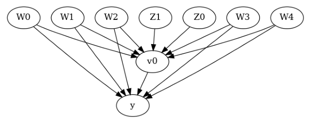
[6]:
from IPython.display import Image, display
display(Image(filename="causal_model.png"))
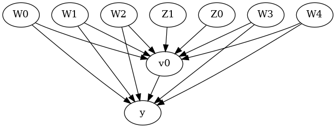
我们得到了一个因果图。现在识别和估计已完成。
[7]:
identified_estimand = model.identify_effect(proceed_when_unidentifiable=True)
print(identified_estimand)
Estimand type: EstimandType.NONPARAMETRIC_ATE

### Estimand : 1
Estimand name: backdoor
Estimand expression:
  d
─────(E[y|W3,W1,W0,W2,W4])
d[v₀]
Estimand assumption 1, Unconfoundedness: If U→{v0} and U→y then P(y|v0,W3,W1,W0,W2,W4,U) = P(y|v0,W3,W1,W0,W2,W4)

### Estimand : 2
Estimand name: iv
Estimand expression:
 ⎡                              -1⎤
 ⎢    d        ⎛    d          ⎞  ⎥
E⎢─────────(y)⋅⎜─────────([v₀])⎟  ⎥
 ⎣d[Z₀  Z₁]    ⎝d[Z₀  Z₁]      ⎠  ⎦
Estimand assumption 1, As-if-random: If U→→y then ¬(U →→{Z0,Z1})
Estimand assumption 2, Exclusion: If we remove {Z0,Z1}→{v0}, then ¬({Z0,Z1}→y)

### Estimand : 3
Estimand name: frontdoor
No such variable(s) found!
方法 1:倾向得分分层#
我们将使用倾向得分对数据中的单元进行分层。
[8]:
causal_estimate_strat = model.estimate_effect(identified_estimand,
                                              method_name="backdoor.propensity_score_stratification",
                                              target_units="att")
print(causal_estimate_strat)
print("Causal Estimate is " + str(causal_estimate_strat.value))
*** Causal Estimate ***

## Identified estimand
Estimand type: EstimandType.NONPARAMETRIC_ATE

### Estimand : 1
Estimand name: backdoor
Estimand expression:
  d
─────(E[y|W3,W1,W0,W2,W4])
d[v₀]
Estimand assumption 1, Unconfoundedness: If U→{v0} and U→y then P(y|v0,W3,W1,W0,W2,W4,U) = P(y|v0,W3,W1,W0,W2,W4)

## Realized estimand
b: y~v0+W3+W1+W0+W2+W4
Target units: att

## Estimate
Mean value: 1.002656737901175

Causal Estimate is 1.002656737901175
文本解释器#
文本解释器(用文字)描述了处理变量单位变化对结果变量的影响。
[9]:
# Textual Interpreter
interpretation = causal_estimate_strat.interpret(method_name="textual_effect_interpreter")
Increasing the treatment variable(s) [v0] from 0 to 1 causes an increase of 1.002656737901175 in the expected value of the outcome [['y']], over the data distribution/population represented by the dataset.
可视化解释器#
可视化解释器绘制了基于倾向得分调整数据集前后,标准化平均差 (SMD) 的变化。SMD 的公式如下所示。
\(SMD = \frac{\bar X_{1} - \bar X_{2}}{\sqrt{(S_{1}^{2} + S_{2}^{2})/2}}\)
此处,\(\bar X_{1}\) 和 \(\bar X_{2}\) 分别是处理组和对照组的样本均值。
[10]:
# Visual Interpreter
interpretation = causal_estimate_strat.interpret(method_name="propensity_balance_interpreter")
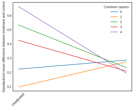
此图显示了 SMD 如何从未调整单位下降到分层单位。
方法 2:倾向得分匹配#
我们将使用倾向得分来匹配数据中的单位。
[11]:
causal_estimate_match = model.estimate_effect(identified_estimand,
                                              method_name="backdoor.propensity_score_matching",
                                              target_units="atc")
print(causal_estimate_match)
print("Causal Estimate is " + str(causal_estimate_match.value))
*** Causal Estimate ***

## Identified estimand
Estimand type: EstimandType.NONPARAMETRIC_ATE

### Estimand : 1
Estimand name: backdoor
Estimand expression:
  d
─────(E[y|W3,W1,W0,W2,W4])
d[v₀]
Estimand assumption 1, Unconfoundedness: If U→{v0} and U→y then P(y|v0,W3,W1,W0,W2,W4,U) = P(y|v0,W3,W1,W0,W2,W4)

## Realized estimand
b: y~v0+W3+W1+W0+W2+W4
Target units: atc

## Estimate
Mean value: 1.0038102718387791

Causal Estimate is 1.0038102718387791
[12]:
# Textual Interpreter
interpretation = causal_estimate_match.interpret(method_name="textual_effect_interpreter")
Increasing the treatment variable(s) [v0] from 0 to 1 causes an increase of 1.0038102718387791 in the expected value of the outcome [['y']], over the data distribution/population represented by the dataset.
此处无法使用倾向平衡解释器,因为该解释器方法仅支持倾向得分分层估计器。
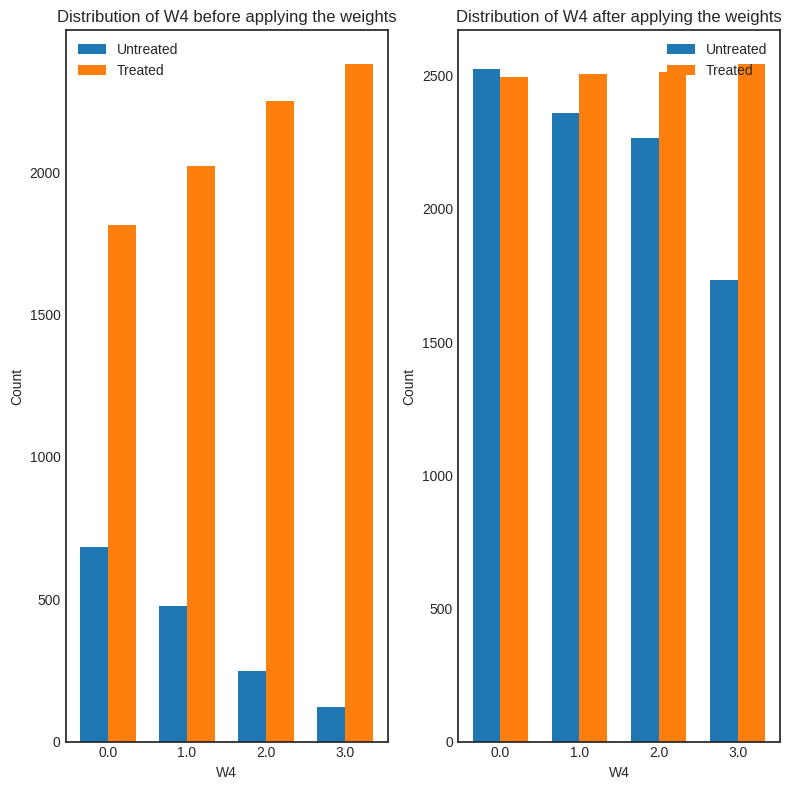
方法 3:加权#
我们将使用(逆向)倾向得分来为数据中的单位分配权重。DoWhy 支持几种不同的加权方案:1. 普通逆倾向得分加权 (IPS) (weighting_scheme=”ips_weight”) 2. 自归一化 IPS 加权(也称为 Hajek 估计器)(weighting_scheme=”ips_normalized_weight”) 3. 稳定化 IPS 加权 (weighting_scheme = “ips_stabilized_weight”)
[13]:
causal_estimate_ipw = model.estimate_effect(identified_estimand,
                                            method_name="backdoor.propensity_score_weighting",
                                            target_units = "ate",
                                            method_params={"weighting_scheme":"ips_weight"})
print(causal_estimate_ipw)
print("Causal Estimate is " + str(causal_estimate_ipw.value))
*** Causal Estimate ***

## Identified estimand
Estimand type: EstimandType.NONPARAMETRIC_ATE

### Estimand : 1
Estimand name: backdoor
Estimand expression:
  d
─────(E[y|W3,W1,W0,W2,W4])
d[v₀]
Estimand assumption 1, Unconfoundedness: If U→{v0} and U→y then P(y|v0,W3,W1,W0,W2,W4,U) = P(y|v0,W3,W1,W0,W2,W4)

## Realized estimand
b: y~v0+W3+W1+W0+W2+W4
Target units: ate

## Estimate
Mean value: 1.2641975291140912

Causal Estimate is 1.2641975291140912
[14]:
# Textual Interpreter
interpretation = causal_estimate_ipw.interpret(method_name="textual_effect_interpreter")
Increasing the treatment variable(s) [v0] from 0 to 1 causes an increase of 1.2641975291140912 in the expected value of the outcome [['y']], over the data distribution/population represented by the dataset.
[15]:
interpretation = causal_estimate_ipw.interpret(method_name="confounder_distribution_interpreter", fig_size=(8,8), font_size=12, var_name='W4', var_type='discrete')
[ ]: