计算因果效应的基础示例#
这是 DoWhy 因果推断库的快速介绍。我们将加载一个样本数据集,并估计预先指定的处理变量对预先指定的结果变量的因果效应。
首先,让我们加载所有必需的软件包。
[1]:
import numpy as np

from dowhy import CausalModel
import dowhy.datasets
现在,让我们加载一个数据集。为简单起见,我们模拟一个数据集,其中公共原因和处理之间、以及公共原因和结果之间存在线性关系。
Beta 是真实的因果效应。
[2]:
data = dowhy.datasets.linear_dataset(beta=10,
        num_common_causes=5,
        num_instruments = 2,
        num_effect_modifiers=1,
        num_samples=5000,
        treatment_is_binary=True,
        stddev_treatment_noise=10,
        num_discrete_common_causes=1)
df = data["df"]
[3]:
df.head()
[3]:
| X0 | Z0 | Z1 | W0 | W1 | W2 | W3 | W4 | v0 | y | |
|---|---|---|---|---|---|---|---|---|---|---|
| 0 | 0.229215 | 1.0 | 0.803310 | 0.969484 | 0.708693 | -0.472480 | 1.134963 | 0 | True | 11.467510 |
| 1 | -1.424967 | 0.0 | 0.163824 | -0.161973 | -0.495899 | -0.971206 | -0.177170 | 0 | False | -2.703782 |
| 2 | 0.462122 | 1.0 | 0.287209 | 2.114670 | -1.484899 | -0.760696 | 1.512796 | 1 | True | 13.401639 |
| 3 | -2.460213 | 0.0 | 0.188397 | 0.524076 | 0.090692 | -1.059184 | -1.477797 | 1 | False | 0.378057 |
| 4 | -2.152985 | 1.0 | 0.276386 | 1.981324 | 0.648104 | -1.882990 | -0.061003 | 0 | True | 9.043652 |
请注意,我们使用 pandas 数据框加载数据。目前,DoWhy 只支持 pandas 数据框作为输入。
接口 1(推荐):输入因果图#
现在我们输入 GML 图格式的因果图(推荐)。您也可以使用 DOT 格式。
要为您的数据集创建因果图,您可以使用像 DAGitty 这样的工具,它提供了一个 GUI 来构建图。您可以导出它生成的图字符串。图字符串与 DOT 格式非常接近:只需将 dag 重命名为 digraph,删除换行符并在每行后添加分号,即可将其转换为 DOT 格式并输入到 DoWhy。
[4]:
# With graph
model=CausalModel(
        data = df,
        treatment=data["treatment_name"],
        outcome=data["outcome_name"],
        graph=data["gml_graph"]
        )
[5]:
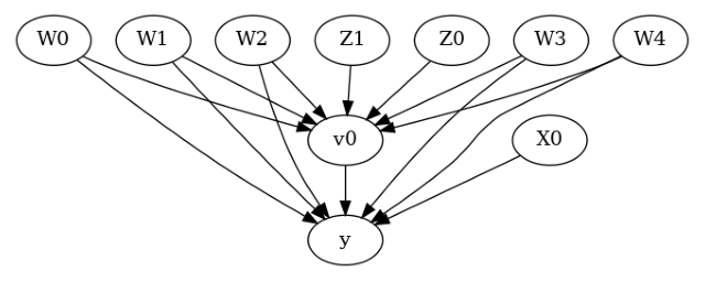
model.view_model()
[6]:
from IPython.display import Image, display
display(Image(filename="causal_model.png"))
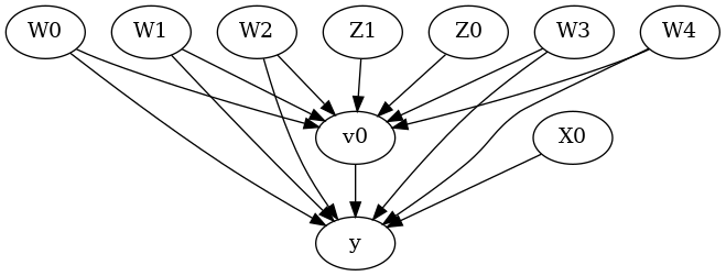
上面的因果图显示了因果模型中编码的假设。我们现在可以使用此图首先识别因果效应(从因果可估量到概率表达式),然后估计因果效应。
DoWhy 理念:将识别和估计分开#
识别可以在不访问数据的情况下实现,仅通过访问图。这会产生一个需要计算的表达式。然后可以在估计步骤中使用可用数据评估此表达式。重要的是要理解这些是正交的步骤。
识别#
[7]:
identified_estimand = model.identify_effect(proceed_when_unidentifiable=True)
print(identified_estimand)
Estimand type: EstimandType.NONPARAMETRIC_ATE

### Estimand : 1
Estimand name: backdoor
Estimand expression:
  d
─────(E[y|W3,W4,W1,W0,W2])
d[v₀]
Estimand assumption 1, Unconfoundedness: If U→{v0} and U→y then P(y|v0,W3,W4,W1,W0,W2,U) = P(y|v0,W3,W4,W1,W0,W2)

### Estimand : 2
Estimand name: iv
Estimand expression:
 ⎡                              -1⎤
 ⎢    d        ⎛    d          ⎞  ⎥
E⎢─────────(y)⋅⎜─────────([v₀])⎟  ⎥
 ⎣d[Z₁  Z₀]    ⎝d[Z₁  Z₀]      ⎠  ⎦
Estimand assumption 1, As-if-random: If U→→y then ¬(U →→{Z1,Z0})
Estimand assumption 2, Exclusion: If we remove {Z1,Z0}→{v0}, then ¬({Z1,Z0}→y)

### Estimand : 3
Estimand name: frontdoor
No such variable(s) found!
注意参数标志 proceed_when_unidentifiable。需要将其设置为 True,以表明我们忽略了任何未观测到的混杂因素。默认行为是提示用户仔细检查是否可以忽略未观测到的混杂因素。
估计#
[8]:
causal_estimate = model.estimate_effect(identified_estimand,
        method_name="backdoor.propensity_score_stratification")
print(causal_estimate)
*** Causal Estimate ***

## Identified estimand
Estimand type: EstimandType.NONPARAMETRIC_ATE

### Estimand : 1
Estimand name: backdoor
Estimand expression:
  d
─────(E[y|W3,W4,W1,W0,W2])
d[v₀]
Estimand assumption 1, Unconfoundedness: If U→{v0} and U→y then P(y|v0,W3,W4,W1,W0,W2,U) = P(y|v0,W3,W4,W1,W0,W2)

## Realized estimand
b: y~v0+W3+W4+W1+W0+W2
Target units: ate

## Estimate
Mean value: 9.666348684992126
您可以向 estimate_effect 方法输入附加参数。例如,要估计对单位的任何子集的影响,您可以指定“target_units”参数,它可以是字符串(“ate”、“att”或“atc”)、过滤数据框行的 lambda 函数,或用于计算效果的新数据框。您还可以指定“effect modifiers”来估计这些变量的异质效应。请参阅 help(CausalModel.estimate_effect)。
[9]:
# Causal effect on the control group (ATC)
causal_estimate_att = model.estimate_effect(identified_estimand,
        method_name="backdoor.propensity_score_stratification",
        target_units = "atc")
print(causal_estimate_att)
print("Causal Estimate is " + str(causal_estimate_att.value))
*** Causal Estimate ***

## Identified estimand
Estimand type: EstimandType.NONPARAMETRIC_ATE

### Estimand : 1
Estimand name: backdoor
Estimand expression:
  d
─────(E[y|W3,W4,W1,W0,W2])
d[v₀]
Estimand assumption 1, Unconfoundedness: If U→{v0} and U→y then P(y|v0,W3,W4,W1,W0,W2,U) = P(y|v0,W3,W4,W1,W0,W2)

## Realized estimand
b: y~v0+W3+W4+W1+W0+W2
Target units: atc

## Estimate
Mean value: 9.670293023783838

Causal Estimate is 9.670293023783838
接口 2:指定公共原因和工具变量#
[10]:
# Without graph
model= CausalModel(
        data=df,
        treatment=data["treatment_name"],
        outcome=data["outcome_name"],
        common_causes=data["common_causes_names"],
        effect_modifiers=data["effect_modifier_names"])
[11]:
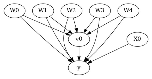
model.view_model()
[12]:
from IPython.display import Image, display
display(Image(filename="causal_model.png"))
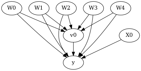
我们得到相同的因果图。现在识别和估计照常进行。
[13]:
identified_estimand = model.identify_effect(proceed_when_unidentifiable=True)
[14]:
estimate = model.estimate_effect(identified_estimand,
                                 method_name="backdoor.propensity_score_stratification")
print(estimate)
print("Causal Estimate is " + str(estimate.value))
*** Causal Estimate ***

## Identified estimand
Estimand type: EstimandType.NONPARAMETRIC_ATE

### Estimand : 1
Estimand name: backdoor
Estimand expression:
  d
─────(E[y|W3,W4,W1,W0,W2])
d[v₀]
Estimand assumption 1, Unconfoundedness: If U→{v0} and U→y then P(y|v0,W3,W4,W1,W0,W2,U) = P(y|v0,W3,W4,W1,W0,W2)

## Realized estimand
b: y~v0+W3+W4+W1+W0+W2
Target units: ate

## Estimate
Mean value: 9.666348684992126

Causal Estimate is 9.666348684992126
驳斥估计值#
现在我们来看看驳斥获得的估计值的方法。驳斥方法提供了每个正确的估计器都应该通过的测试。因此,如果一个估计器未能通过驳斥测试(p 值 <0.05),则意味着该估计器存在一些问题。
请注意,我们无法验证估计值是否正确,但如果它违反了某些预期行为,我们可以拒绝它(这类似于科学理论可以被证伪但不能被证明为真)。以下驳斥测试基于以下两种方法:1) 不变变换:数据中的变化不应改变估计值。任何结果在原始数据和修改后的数据之间显著变化的估计器都未能通过测试;
随机公共原因
数据子集
无效变换:数据更改后,真实的因果估计值为零。任何在新数据上结果与零显著不同的估计器都未能通过测试。
安慰剂处理
添加一个随机公共原因变量#
[15]:
res_random=model.refute_estimate(identified_estimand, estimate, method_name="random_common_cause", show_progress_bar=True)
print(res_random)
Refute: Add a random common cause
Estimated effect:9.666348684992126
New effect:9.66634868499213
p value:1.0
用随机(安慰剂)变量替换处理#
[16]:
res_placebo=model.refute_estimate(identified_estimand, estimate,
        method_name="placebo_treatment_refuter", show_progress_bar=True, placebo_type="permute")
print(res_placebo)
Refute: Use a Placebo Treatment
Estimated effect:9.666348684992126
New effect:0.029698445089780416
p value:0.94
移除数据的随机子集#
[17]:
res_subset=model.refute_estimate(identified_estimand, estimate,
        method_name="data_subset_refuter", show_progress_bar=True, subset_fraction=0.9)
print(res_subset)
Refute: Use a subset of data
Estimated effect:9.666348684992126
New effect:9.702493576161388
p value:0.5800000000000001
如您所见,倾向得分分层估计器对驳斥具有相当强的鲁棒性。
可复现性:为了可复现性,您可以向任何驳斥方法添加一个参数“random_seed”,如下所示。
并行化:您还可以使用内置并行化来加速驳斥过程。只需将 n_jobs 设置为大于 1 的值,即可将工作负载分散到多个 CPU;或将 n_jobs=-1 设置为使用所有 CPU。目前,此功能仅适用于 random_common_cause、placebo_treatment_refuter 和 data_subset_refuter。
[18]:
res_subset=model.refute_estimate(identified_estimand, estimate,
        method_name="data_subset_refuter", show_progress_bar=True, subset_fraction=0.9, random_seed = 1, n_jobs=-1, verbose=10)
print(res_subset)
[Parallel(n_jobs=-1)]: Using backend LokyBackend with 4 concurrent workers.
[Parallel(n_jobs=-1)]: Done   5 tasks      | elapsed:    3.1s
[Parallel(n_jobs=-1)]: Done  10 tasks      | elapsed:    3.6s
[Parallel(n_jobs=-1)]: Done  17 tasks      | elapsed:    4.4s
[Parallel(n_jobs=-1)]: Done  24 tasks      | elapsed:    4.9s
[Parallel(n_jobs=-1)]: Done  33 tasks      | elapsed:    6.0s
[Parallel(n_jobs=-1)]: Done  42 tasks      | elapsed:    6.9s
[Parallel(n_jobs=-1)]: Done  53 tasks      | elapsed:    8.1s
[Parallel(n_jobs=-1)]: Done  64 tasks      | elapsed:    9.1s
[Parallel(n_jobs=-1)]: Done  77 tasks      | elapsed:   10.6s
[Parallel(n_jobs=-1)]: Done  90 tasks      | elapsed:   12.0s
Refute: Use a subset of data
Estimated effect:9.666348684992126
New effect:9.701936861633671
p value:0.6000000000000001
[Parallel(n_jobs=-1)]: Done 100 out of 100 | elapsed: 12.9s finished
添加一个未观测到的公共原因变量#
此驳斥不返回 p 值。相反,它提供了一个敏感性测试,以了解如果识别假设(在 identify_effect 中使用)无效,估计值会以多快的速度变化。具体来说,它检查对违反后门假设的敏感性:即所有公共原因都被观测到。
为此,它创建一个新数据集,其中在处理和结果之间添加了一个公共原因。为了捕捉公共原因的影响,该方法将公共原因对处理和结果影响的强度作为输入。根据这些关于公共原因影响的输入,它会改变处理和结果值,然后重新运行估计器。希望新的估计值不会因未观测到的公共原因的微小影响而发生剧烈变化,这表明对任何未观测到的混杂因素都具有鲁棒性。
解释此过程的另一种等效方法是假设输入数据中已经存在未观测到的混杂因素。处理和结果值的变化消除了原始数据中存在的任何未观测到的公共原因的影响。然后在修改后的数据上重新运行估计器可以提供正确的识别估计值,我们希望新估计值与原始估计值之间的差异不要太大,对于未观测到的公共原因影响的某个有界值而言。
领域知识的重要性:此测试需要领域知识来设置未观测到的混杂因素影响的合理输入值。我们首先展示混杂因素对处理和结果影响的单一值的结果。
[19]:
res_unobserved=model.refute_estimate(identified_estimand, estimate, method_name="add_unobserved_common_cause",
                                     confounders_effect_on_treatment="binary_flip", confounders_effect_on_outcome="linear",
                                    effect_strength_on_treatment=0.01, effect_strength_on_outcome=0.02)
print(res_unobserved)
Refute: Add an Unobserved Common Cause
Estimated effect:9.666348684992126
New effect:8.664434813571749
通常更有用的是检查随着未观测到的混杂因素影响增加的趋势。为此,我们可以提供一系列假设的混杂因素影响。输出是不同未观测到的混杂因素下估计效应的(最小值,最大值)范围。
[20]:
res_unobserved_range=model.refute_estimate(identified_estimand, estimate, method_name="add_unobserved_common_cause",
                                     confounders_effect_on_treatment="binary_flip", confounders_effect_on_outcome="linear",
                                    effect_strength_on_treatment=np.array([0.001, 0.005, 0.01, 0.02]), effect_strength_on_outcome=0.01)
print(res_unobserved_range)
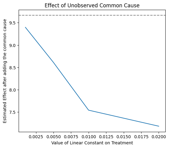
Refute: Add an Unobserved Common Cause
Estimated effect:9.666348684992126
New effect:(7.184834387565013, 9.395788216420343)
上图显示了随着假设的对处理的混杂影响增加,估计值如何降低。通过领域知识,我们可能知道对处理的最大可能混杂影响。由于我们看到影响没有超出零,我们可以安全地得出结论,处理 v0 的因果效应是正向的。
我们还可以改变对处理和结果的混杂影响。我们得到一个热力图。
[21]:
res_unobserved_range=model.refute_estimate(identified_estimand, estimate, method_name="add_unobserved_common_cause",
                                           confounders_effect_on_treatment="binary_flip", confounders_effect_on_outcome="linear",
                                           effect_strength_on_treatment=[0.001, 0.005, 0.01, 0.02],
                                           effect_strength_on_outcome=[0.001, 0.005, 0.01,0.02])
print(res_unobserved_range)
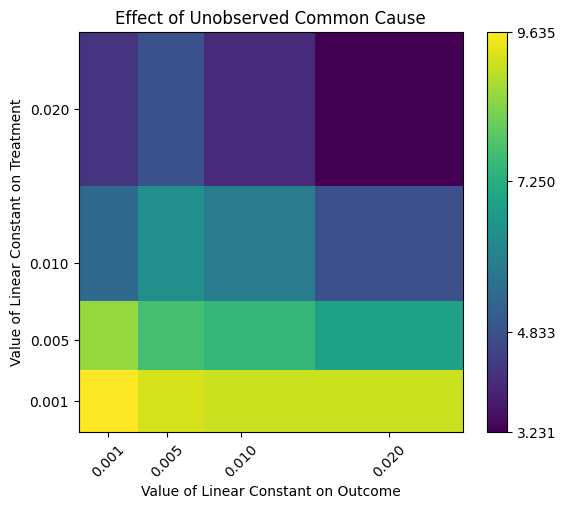
Refute: Add an Unobserved Common Cause
Estimated effect:9.666348684992126
New effect:(3.2311645505216724, 9.63495028468222)
自动推断影响强度参数。 最后,DoWhy 支持自动选择影响强度参数。这基于一个假设:未观测到的混杂因素对处理或结果的影响不会强于任何已观测到的混杂因素。也就是说,我们至少已经收集了与最相关的混杂因素相关的数据。如果是这样,那么我们可以通过已观测到的混杂因素的影响强度来限制 effect_strength_on_treatment 和 effect_strength_on_outcome 的范围。还有一个可选参数,用于指示未观测到的混杂因素的影响强度是否应该与最高已观测到的影响强度一样高,或者只是其中的一部分。您可以使用可选的 effect_fraction_on_treatment 和 effect_fraction_on_outcome 参数进行设置。默认情况下,这两个参数都是 1。
[22]:
res_unobserved_auto = model.refute_estimate(identified_estimand, estimate, method_name="add_unobserved_common_cause",
                                           confounders_effect_on_treatment="binary_flip", confounders_effect_on_outcome="linear")
print(res_unobserved_auto)
/github/home/.cache/pypoetry/virtualenvs/dowhy-oN2hW5jr-py3.8/lib/python3.8/site-packages/sklearn/utils/validation.py:1183: DataConversionWarning: A column-vector y was passed when a 1d array was expected. Please change the shape of y to (n_samples, ), for example using ravel().
  y = column_or_1d(y, warn=True)
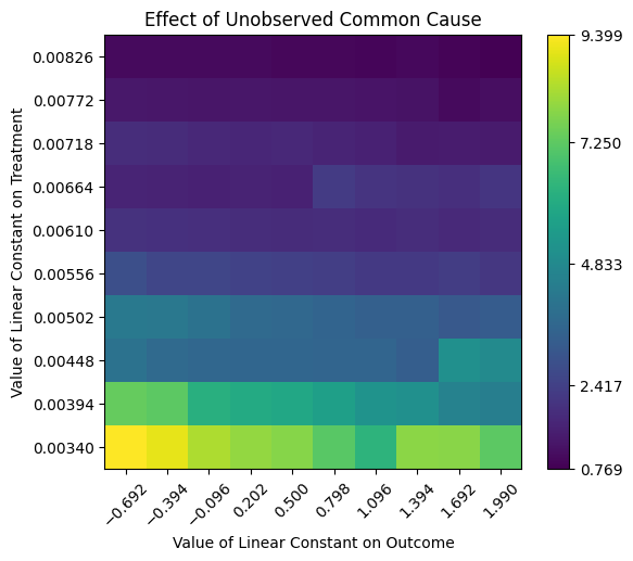
Refute: Add an Unobserved Common Cause
Estimated effect:9.666348684992126
New effect:(0.7690576672487185, 9.398648715588278)
结论:假设未观测到的混杂因素对处理或结果的影响不强于任何已观测到的混杂因素,则可以得出结论,因果效应是正向的。