图形因果模型的基本示例#
步骤 1:将因果关系建模为结构因果模型 (SCM)#
第一步是将与我们的用例相关的变量之间的因果关系建模。我们以因果图的形式进行建模。因果图是一个有向无环图 (DAG),其中边 X→Y 表示 X 导致 Y。从统计学上讲,因果图编码了变量之间的条件独立性关系。使用 NetworkX 库,我们可以创建因果图。在下面的代码片段中,我们创建了一个链 X→Y→Z
[1]:
import networkx as nx
causal_graph = nx.DiGraph([('X', 'Y'), ('Y', 'Z')])
为了使用因果图回答因果问题,我们还需要了解变量底层数据生成过程的性质。因果图本身作为一种图示,不包含有关数据生成过程的任何信息。为了引入这种数据生成过程,我们使用了构建在因果图之上的 SCM
[2]:
from dowhy import gcm
causal_model = gcm.StructuralCausalModel(causal_graph)
此时我们通常会加载我们的数据集。作为本介绍的一部分,我们生成一些合成数据。API 接受 Pandas DataFrame 形式的数据
[3]:
import numpy as np, pandas as pd

X = np.random.normal(loc=0, scale=1, size=1000)
Y = 2 * X + np.random.normal(loc=0, scale=1, size=1000)
Z = 3 * Y + np.random.normal(loc=0, scale=1, size=1000)
data = pd.DataFrame(data=dict(X=X, Y=Y, Z=Z))
data.head()
[3]:
| X | Y | Z | |
|---|---|---|---|
| 0 | -0.748585 | -2.775036 | -5.522909 |
| 1 | 0.304654 | 0.606429 | 1.369306 |
| 2 | -0.214986 | -1.052285 | -3.247393 |
| 3 | -1.057319 | -3.664262 | -10.329441 |
| 4 | -1.875360 | -3.642252 | -12.891059 |
请注意,列 X、Y、Z 与上面构建的图中的节点 X、Y、Z 相对应。我们还可以看到在该数据集中,X 的值如何影响 Y 的值,以及 Y 的值如何影响 Z 的值。
上面创建的因果模型现在允许我们以函数式因果模型的形式为每个节点分配因果机制。在这里,如果事先了解某些因果关系,可以手动分配这些机制;或者也可以使用 auto 模块自动分配。对于后者,我们只需调用
[4]:
auto_assignment_summary = gcm.auto.assign_causal_mechanisms(causal_model, data)
可选地,我们可以从自动分配过程中获得更多见解
[5]:
print(auto_assignment_summary)
When using this auto assignment function, the given data is used to automatically assign a causal mechanism to each node. Note that causal mechanisms can also be customized and assigned manually.
The following types of causal mechanisms are considered for the automatic selection:

If root node:
An empirical distribution, i.e., the distribution is represented by randomly sampling from the provided data. This provides a flexible and non-parametric way to model the marginal distribution and is valid for all types of data modalities.

If non-root node and the data is continuous:
Additive Noise Models (ANM) of the form X_i = f(PA_i) + N_i, where PA_i are the parents of X_i and the unobserved noise N_i is assumed to be independent of PA_i.To select the best model for f, different regression models are evaluated and the model with the smallest mean squared error is selected.Note that minimizing the mean squared error here is equivalent to selecting the best choice of an ANM.

If non-root node and the data is discrete:
Discrete Additive Noise Models have almost the same definition as non-discrete ANMs, but come with an additional constraint for f to only return discrete values.
Note that 'discrete' here refers to numerical values with an order. If the data is categorical, consider representing them as strings to ensure proper model selection.

If non-root node and the data is categorical:
A functional causal model based on a classifier, i.e., X_i = f(PA_i, N_i).
Here, N_i follows a uniform distribution on [0, 1] and is used to randomly sample a class (category) using the conditional probability distribution produced by a classification model.Here, different model classes are evaluated using the (negative) F1 score and the best performing model class is selected.

In total, 3 nodes were analyzed:

--- Node: X
Node X is a root node. Therefore, assigning 'Empirical Distribution' to the node representing the marginal distribution.

--- Node: Y
Node Y is a non-root node with continuous data. Assigning 'AdditiveNoiseModel using LinearRegression' to the node.
This represents the causal relationship as Y := f(X) + N.
For the model selection, the following models were evaluated on the mean squared error (MSE) metric:
LinearRegression: 0.9800842672468573
Pipeline(steps=[('polynomialfeatures', PolynomialFeatures(include_bias=False)),
                ('linearregression', LinearRegression)]): 0.9838556091349311
HistGradientBoostingRegressor: 1.1417205950883154

--- Node: Z
Node Z is a non-root node with continuous data. Assigning 'AdditiveNoiseModel using LinearRegression' to the node.
This represents the causal relationship as Z := f(Y) + N.
For the model selection, the following models were evaluated on the mean squared error (MSE) metric:
LinearRegression: 0.967971347157131
Pipeline(steps=[('polynomialfeatures', PolynomialFeatures(include_bias=False)),
                ('linearregression', LinearRegression)]): 0.9711734724588762
HistGradientBoostingRegressor: 1.4150521077422746

===Note===
Note, based on the selected auto assignment quality, the set of evaluated models changes.
For more insights toward the quality of the fitted graphical causal model, consider using the evaluate_causal_model function after fitting the causal mechanisms.
如果想对分配的机制有更多控制权,也可以手动进行。例如,我们可以将经验分布分配给根节点 X,并将线性加性噪声模型分配给节点 Y 和 Z
[6]:
causal_model.set_causal_mechanism('X', gcm.EmpiricalDistribution())
causal_model.set_causal_mechanism('Y', gcm.AdditiveNoiseModel(gcm.ml.create_linear_regressor()))
causal_model.set_causal_mechanism('Z', gcm.AdditiveNoiseModel(gcm.ml.create_linear_regressor()))
在这里,我们将节点 X 设置为遵循我们观察到的经验分布(非参数),并将节点 Y 和 Z 设置为遵循明确设定线性关系的加性噪声模型。
在现实世界中,数据是以不透明的值流形式出现的,我们通常不知道一个变量如何影响另一个变量。图形因果模型可以帮助我们重新解构这些因果关系,即使我们之前并不了解它们。
步骤 2:将 SCM 与数据拟合#
有了手头的数据和之前构建的图,我们现在可以使用 fit 训练 SCM
[7]:
gcm.fit(causal_model, data)
Fitting causal mechanism of node Z: 100%|██████████| 3/3 [00:00<00:00, 517.77it/s]
拟合意味着,我们根据数据学习 SCM 中变量的生成模型。
拟合完成后,我们还可以获得更多关于模型性能的见解
[8]:
print(gcm.evaluate_causal_model(causal_model, data))
Evaluating causal mechanisms...: 100%|██████████| 3/3 [00:00<00:00, 3930.93it/s]
Test permutations of given graph: 100%|██████████| 6/6 [00:00<00:00, 19.98it/s]
Evaluated the performance of the causal mechanisms and the invertibility assumption of the causal mechanisms and the overall average KL divergence between generated and observed distribution and the graph structure. The results are as follows:
==== Evaluation of Causal Mechanisms ====
The used evaluation metrics are:
- KL divergence (only for root-nodes): Evaluates the divergence between the generated and the observed distribution.
- Mean Squared Error (MSE): Evaluates the average squared differences between the observed values and the conditional expectation of the causal mechanisms.
- Normalized MSE (NMSE): The MSE normalized by the standard deviation for better comparison.
- R2 coefficient: Indicates how much variance is explained by the conditional expectations of the mechanisms. Note, however, that this can be misleading for nonlinear relationships.
- F1 score (only for categorical non-root nodes): The harmonic mean of the precision and recall indicating the goodness of the underlying classifier model.
- (normalized) Continuous Ranked Probability Score (CRPS): The CRPS generalizes the Mean Absolute Percentage Error to probabilistic predictions. This gives insights into the accuracy and calibration of the causal mechanisms.
NOTE: Every metric focuses on different aspects and they might not consistently indicate a good or bad performance.
We will mostly utilize the CRPS for comparing and interpreting the performance of the mechanisms, since this captures the most important properties for the causal model.
--- Node X
- The KL divergence between generated and observed distribution is 0.01649976739835941.
The estimated KL divergence indicates an overall very good representation of the data distribution.
--- Node Y
- The MSE is 0.9815044724137867.
- The NMSE is 0.45008485875858045.
- The R2 coefficient is 0.7964232578341484.
- The normalized CRPS is 0.25767351203525335.
The estimated CRPS indicates a good model performance.
--- Node Z
- The MSE is 0.9744960250422121.
- The NMSE is 0.14769619730165157.
- The R2 coefficient is 0.9781428218637729.
- The normalized CRPS is 0.08464191146545343.
The estimated CRPS indicates a very good model performance.
==== Evaluation of Invertible Functional Causal Model Assumption ====
--- The model assumption for node Y is not rejected with a p-value of 1.0 (after potential adjustment) and a significance level of 0.05.
This implies that the model assumption might be valid.
--- The model assumption for node Z is not rejected with a p-value of 1.0 (after potential adjustment) and a significance level of 0.05.
This implies that the model assumption might be valid.
Note that these results are based on statistical independence tests, and the fact that the assumption was not rejected does not necessarily imply that it is correct. There is just no evidence against it.
==== Evaluation of Generated Distribution ====
The overall average KL divergence between the generated and observed distribution is 0.025964440393727767
The estimated KL divergence indicates an overall very good representation of the data distribution.
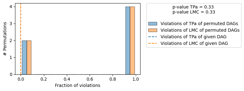
==== Evaluation of the Causal Graph Structure ====
+-------------------------------------------------------------------------------------------------------+
| Falsification Summary |
+-------------------------------------------------------------------------------------------------------+
| The given DAG is not informative because 2 / 6 of the permutations lie in the Markov |
| equivalence class of the given DAG (p-value: 0.33). |
| The given DAG violates 0/1 LMCs and is better than 66.7% of the permuted DAGs (p-value: 0.33). |
| Based on the provided significance level (0.2) and because the DAG is not informative, |
| we do not reject the DAG. |
+-------------------------------------------------------------------------------------------------------+
==== NOTE ====
Always double check the made model assumptions with respect to the graph structure and choice of causal mechanisms.
All these evaluations give some insight into the goodness of the causal model, but should not be overinterpreted, since some causal relationships can be intrinsically hard to model. Furthermore, many algorithms are fairly robust against misspecifications or poor performances of causal mechanisms.
这个摘要告诉我们几点: - 我们的模型拟合得很好。 - 加性噪声模型假设没有被拒绝。 - 生成的分布与观测到的分布非常相似。 - 因果图结构没有被拒绝。
请注意,此评估可能需要相当长的时间,具体取决于模型的复杂性、图的大小和数据量。为了加快速度,请考虑更改评估参数。
步骤 3:基于 SCM 回答因果查询#
最后一步,回答因果问题,是我们的实际目标。例如,我们可以问“如果我干预 Y,变量 Z 会发生什么变化?”
这可以通过 interventional_samples 函数完成。方法如下
[9]:
samples = gcm.interventional_samples(causal_model,
                                     {'Y': lambda y: 2.34 },
                                     num_samples_to_draw=1000)
samples.head()
[9]:
| X | Y | Z | |
|---|---|---|---|
| 0 | -0.416965 | 2.34 | 6.447330 |
| 1 | -0.389357 | 2.34 | 4.558476 |
| 2 | -0.167646 | 2.34 | 6.304203 |
| 3 | -0.114846 | 2.34 | 5.991273 |
| 4 | -1.158345 | 2.34 | 7.103817 |
这个干预表示:“我将忽略 X 对 Y 的任何因果效应,并将 Y 的每个值都设置为 2.34。” 因此,X 的分布将保持不变,而 Y 的值将是一个固定值,Z 将根据其因果模型做出响应。
DoWhy 提供了广泛的因果问题,可以使用 GCM 回答。更多示例请参阅用户指南或其他 Notebooks。