因果发现示例

本 Notebook 的目标是展示因果发现方法如何与 DoWhy 配合使用。我们使用来自 causal-learn 仓库的发现方法。正如我们将看到的，因果发现方法需要适当的假设才能保证正确性，因此在实践中，不同方法返回的结果会有差异。然而，这些方法可以与领域知识有效地结合起来，以构建最终的因果图。

import dowhy
from dowhy import CausalModel

import numpy as np
import pandas as pd
import graphviz
import networkx as nx

np.set_printoptions(precision=3, suppress=True)
np.random.seed(0)

工具函数

我们定义一个工具函数来绘制有向无环图。

def make_graph(adjacency_matrix, labels=None):
    idx = np.abs(adjacency_matrix) > 0.01
    dirs = np.where(idx)
    d = graphviz.Digraph(engine='dot')
    names = labels if labels else [f'x{i}' for i in range(len(adjacency_matrix))]
    for name in names:
        d.node(name)
    for to, from_, coef in zip(dirs[0], dirs[1], adjacency_matrix[idx]):
        d.edge(names[from_], names[to], label=str(coef))
    return d

def str_to_dot(string):
    '''
    Converts input string from graphviz library to valid DOT graph format.
    '''
    graph = string.strip().replace('\n', ';').replace('\t','')
    graph = graph[:9] + graph[10:-2] + graph[-1] # Removing unnecessary characters from string
    return graph

Auto-MPG 数据集实验

在本节中，我们将使用一个包含汽车技术规范的数据集。该数据集从 UCI 机器学习库下载。数据集包含 9 个属性和 398 个实例。我们不知道该数据集的真实因果图，将使用 causal-learn 来发现它。然后将获得的因果图用于估算因果效应。

1. 加载数据

# Load a modified version of the Auto MPG data: Quinlan,R.. (1993). Auto MPG. UCI Machine Learning Repository. https://doi.org/10.24432/C5859H.
data_mpg = pd.read_csv("datasets/auto_mpg.csv", index_col=0)

print(data_mpg.shape)
data_mpg.head()

(392, 6)

	mpg	气缸数	排量	马力	重量	加速度
0	18.0	8.0	307.0	130.0	3504.0	12.0
1	15.0	8.0	350.0	165.0	3693.0	11.5
2	18.0	8.0	318.0	150.0	3436.0	11.0
3	16.0	8.0	304.0	150.0	3433.0	12.0
4	17.0	8.0	302.0	140.0	3449.0	10.5

使用 causal-learn 进行因果发现

我们使用 causal-learn 库对 Auto-MPG 数据集进行因果发现。此处我们使用三种因果发现方法：PC、GES 和 LiNGAM。这些方法被广泛使用且运行时间不长。因此，它们非常适合作为该主题的介绍。Causal-learn 提供了经过充分测试的因果发现方法的完整列表，欢迎读者探索。

所用方法的文档如下： - PC [链接] - GES [链接] - LiNGAM [链接]

更多方法可在 causal-learn 文档中找到 [链接]。

我们首先尝试使用默认参数的 PC 算法。

from causallearn.search.ConstraintBased.PC import pc

labels = [f'{col}' for i, col in enumerate(data_mpg.columns)]
data = data_mpg.to_numpy()

cg = pc(data)

# Visualization using pydot
from causallearn.utils.GraphUtils import GraphUtils
import matplotlib.image as mpimg
import matplotlib.pyplot as plt
import io

pyd = GraphUtils.to_pydot(cg.G, labels=labels)
tmp_png = pyd.create_png(f="png")
fp = io.BytesIO(tmp_png)
img = mpimg.imread(fp, format='png')
plt.axis('off')
plt.imshow(img)
plt.show()

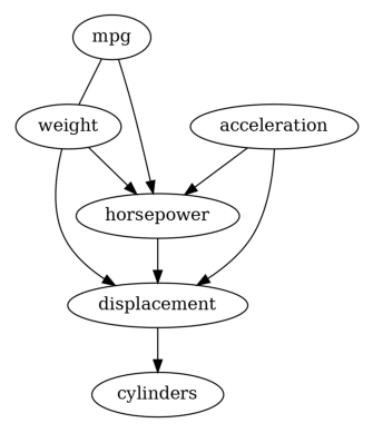
然后我们得到了 PC 发现的因果图。我们也试试 GES 看看结果。

from causallearn.search.ScoreBased.GES import ges

# default parameters
Record = ges(data)

# Visualization using pydot
from causallearn.utils.GraphUtils import GraphUtils
import matplotlib.image as mpimg
import matplotlib.pyplot as plt
import io

pyd = GraphUtils.to_pydot(Record['G'], labels=labels)
tmp_png = pyd.create_png(f="png")
fp = io.BytesIO(tmp_png)
img = mpimg.imread(fp, format='png')
plt.axis('off')
plt.imshow(img)
plt.show()

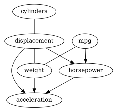
嗯，这两个结果是不同的，这在将因果发现应用于真实世界数据集时并不少见，因为对数据生成过程所需的假设很难验证。

此外，PC 和 GES 返回的图是 CPDAGs 而不是 DAGs，因此可能存在无向边（例如，GES 返回的结果）。因此，对于这些方法来说，因果效应估计很困难，因为可能缺乏后门变量、工具变量或前门变量。为了获得 DAG，我们决定在我们的数据集上尝试 LiNGAM。

from causallearn.search.FCMBased import lingam
model_lingam = lingam.ICALiNGAM()
model_lingam.fit(data)

from causallearn.search.FCMBased.lingam.utils import make_dot
make_dot(model_lingam.adjacency_matrix_, labels=labels)

现在我们有了 DAG，并准备好基于此估算因果效应。

使用线性回归估算因果效应

现在让我们看看 mpg 对 weight 的因果效应估算。

# Obtain valid dot format
graph_dot = make_graph(model_lingam.adjacency_matrix_, labels=labels)

# Define Causal Model
model=CausalModel(
        data = data_mpg,
        treatment='mpg',
        outcome='weight',
        graph=str_to_dot(graph_dot.source))

# Identification
identified_estimand = model.identify_effect(proceed_when_unidentifiable=True)
print(identified_estimand)

# Estimation
estimate = model.estimate_effect(identified_estimand,
                                method_name="backdoor.linear_regression",
                                control_value=0,
                                treatment_value=1,
                                confidence_intervals=True,
                                test_significance=True)
print("Causal Estimate is " + str(estimate.value))

Estimand type: EstimandType.NONPARAMETRIC_ATE

### Estimand : 1
Estimand name: backdoor
Estimand expression:
  d
──────(E[weight|cylinders])
d[mpg]
Estimand assumption 1, Unconfoundedness: If U→{mpg} and U→weight then P(weight|mpg,cylinders,U) = P(weight|mpg,cylinders)

### Estimand : 2
Estimand name: iv
No such variable(s) found!

### Estimand : 3
Estimand name: frontdoor
No such variable(s) found!

Causal Estimate is -38.94097365620928

Sachs 数据集实验

该数据集包含同时测量了从数千个单独的原代免疫系统细胞中提取的 11 种磷酸化蛋白质和磷脂，这些细胞经历了通用和特定的分子干预（Sachs 等人，2005 年）。

数据集的规格如下： - 节点数：11 - 弧数：17 - 参数数：178 - 平均马尔可夫毯大小：3.09 - 平均度数：3.09 - 最大入度：3 - 实例数：7466

1. 加载数据

from causallearn.utils.Dataset import load_dataset

data_sachs, labels = load_dataset("sachs")

print(data_sachs.shape)
print(labels)

(7466, 11)
['raf', 'mek', 'plc', 'pip2', 'pip3', 'erk', 'akt', 'pka', 'pkc', 'p38', 'jnk']

使用 causal-learn 进行因果发现

我们使用上面提到的三种因果发现方法（PC、GES 和 LiNGAM）来寻找因果图。

首先，让我们看看 PC 是如何工作的。

graphs = {}
graphs_nx = {}
labels = [f'{col}' for i, col in enumerate(labels)]
data = data_sachs

from causallearn.search.ConstraintBased.PC import pc

cg = pc(data)

# Visualization using pydot
from causallearn.utils.GraphUtils import GraphUtils
import matplotlib.image as mpimg
import matplotlib.pyplot as plt
import io

pyd = GraphUtils.to_pydot(cg.G, labels=labels)
tmp_png = pyd.create_png(f="png")
fp = io.BytesIO(tmp_png)
img = mpimg.imread(fp, format='png')
plt.axis('off')
plt.imshow(img)
plt.show()

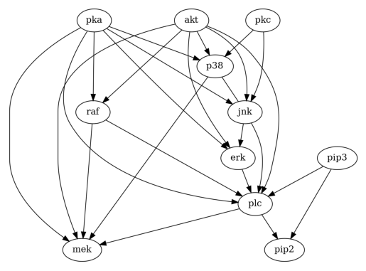
然后，我们试试 GES。

from causallearn.search.ScoreBased.GES import ges

# default parameters
Record = ges(data)

# Visualization using pydot
from causallearn.utils.GraphUtils import GraphUtils
import matplotlib.image as mpimg
import matplotlib.pyplot as plt
import io

pyd = GraphUtils.to_pydot(Record['G'], labels=labels)
tmp_png = pyd.create_png(f="png")
fp = io.BytesIO(tmp_png)
img = mpimg.imread(fp, format='png')
plt.axis('off')
plt.imshow(img)
plt.show()

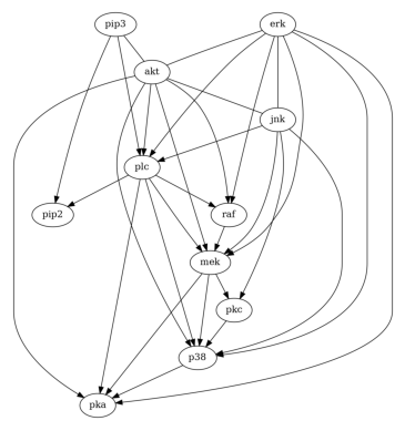
还有 LiNGAM。

from causallearn.search.FCMBased import lingam
model = lingam.ICALiNGAM()
model.fit(data)

from causallearn.search.FCMBased.lingam.utils import make_dot
make_dot(model.adjacency_matrix_, labels=labels)

使用线性回归估算效应

类似地，让我们使用 LiNGAM 返回的 DAG 来估算 PIP2 对 PKC 的因果效应。

# Obtain valid dot format
graph_dot = make_graph(model.adjacency_matrix_, labels=labels)

data_df = pd.DataFrame(data=data, columns=labels)

# Define Causal Model
model_est=CausalModel(
        data = data_df,
        treatment='pip2',
        outcome='pkc',
        graph=str_to_dot(graph_dot.source))

# Identification
identified_estimand = model_est.identify_effect(proceed_when_unidentifiable=False)
print(identified_estimand)

# Estimation
estimate = model_est.estimate_effect(identified_estimand,
                                method_name="backdoor.linear_regression",
                                control_value=0,
                                treatment_value=1,
                                confidence_intervals=True,
                                test_significance=True)
print("Causal Estimate is " + str(estimate.value))

Estimand type: EstimandType.NONPARAMETRIC_ATE

### Estimand : 1
Estimand name: backdoor
Estimand expression:
   d
───────(E[pkc|plc,pip3])
d[pip₂]
Estimand assumption 1, Unconfoundedness: If U→{pip2} and U→pkc then P(pkc|pip2,plc,pip3,U) = P(pkc|pip2,plc,pip3)

### Estimand : 2
Estimand name: iv
No such variable(s) found!

### Estimand : 3
Estimand name: frontdoor
No such variable(s) found!

Causal Estimate is 0.033971892284519356