对 Lalonde 和 IHDP 数据集应用反驳测试#
导入依赖项#
[1]:
import dowhy
from dowhy import CausalModel
import pandas as pd
import numpy as np

# Config dict to set the logging level
import logging.config
DEFAULT_LOGGING = {
    'version': 1,
    'disable_existing_loggers': False,
    'loggers': {
        '': {
            'level': 'WARN',
        },
    }
}

logging.config.dictConfig(DEFAULT_LOGGING)
# Disabling warnings output
import warnings
from sklearn.exceptions import DataConversionWarning
warnings.filterwarnings(action='ignore', category=DataConversionWarning)
加载数据集#
婴儿健康和发展计划数据集 (IHDP)#
使用的测量指标包括:儿童的出生体重、头围、早产周数、出生顺序、是否头胎、新生儿健康指数(参见 Scott 和 Bauer 1989)、性别、是否双胞胎——以及母亲在怀孕期间的行为——是否吸烟、饮酒、服药——以及母亲在分娩时的测量指标——年龄、婚姻状况、教育程度(未高中毕业、高中毕业、上过大学但未毕业、大学毕业)、怀孕期间是否工作、是否接受产前护理——以及家庭开始干预时所在的地点(共 8 个)。数据包含 6 个连续协变量和 19 个二元协变量。
参考文献#
Hill, J. L. (2011). Bayesian nonparametric modeling for causal inference. Journal of Computational and Graphical Statistics, 20(1), 217-240. https://doi.org/10.1198/jcgs.2010.08162
[2]:
data = pd.read_csv("https://raw.githubusercontent.com/AMLab-Amsterdam/CEVAE/master/datasets/IHDP/csv/ihdp_npci_1.csv", header = None)
col =  ["treatment", "y_factual", "y_cfactual", "mu0", "mu1" ,]
for i in range(1,26):
    col.append("x"+str(i))
data.columns = col
data = data.astype({"treatment":'bool'}, copy=False)
data.head()
[2]:
| treatment | y_factual | y_cfactual | mu0 | mu1 | x1 | x2 | x3 | x4 | x5 | ... | x16 | x17 | x18 | x19 | x20 | x21 | x22 | x23 | x24 | x25 | |
|---|---|---|---|---|---|---|---|---|---|---|---|---|---|---|---|---|---|---|---|---|---|
| 0 | True | 5.599916 | 4.318780 | 3.268256 | 6.854457 | -0.528603 | -0.343455 | 1.128554 | 0.161703 | -0.316603 | ... | 1 | 1 | 1 | 1 | 0 | 0 | 0 | 0 | 0 | 0 |
| 1 | False | 6.875856 | 7.856495 | 6.636059 | 7.562718 | -1.736945 | -1.802002 | 0.383828 | 2.244320 | -0.629189 | ... | 1 | 1 | 1 | 1 | 0 | 0 | 0 | 0 | 0 | 0 |
| 2 | False | 2.996273 | 6.633952 | 1.570536 | 6.121617 | -0.807451 | -0.202946 | -0.360898 | -0.879606 | 0.808706 | ... | 1 | 0 | 1 | 1 | 0 | 0 | 0 | 0 | 0 | 0 |
| 3 | False | 1.366206 | 5.697239 | 1.244738 | 5.889125 | 0.390083 | 0.596582 | -1.850350 | -0.879606 | -0.004017 | ... | 1 | 0 | 1 | 1 | 0 | 0 | 0 | 0 | 0 | 0 |
| 4 | False | 1.963538 | 6.202582 | 1.685048 | 6.191994 | -1.045229 | -0.602710 | 0.011465 | 0.161703 | 0.683672 | ... | 1 | 1 | 1 | 1 | 0 | 0 | 0 | 0 | 0 | 0 |
5 行 × 30 列
Lalonde 数据集#
一个包含 445 个观测值和以下 12 个变量的数据框。
age:年龄(岁)。
educ:受教育年限。
black:黑人指示变量。
hisp:西班牙裔指示变量。
married:婚姻状况指示变量。
nodegr:高中毕业文凭指示变量。
re74:1974 年实际收入。
re75:1975 年实际收入。
re78:1978 年实际收入。
u74:1974 年收入为零的指示变量。
u75:1975 年收入为零的指示变量。
treat:治疗状态的指示变量。
参考文献#
Dehejia, Rajeev and Sadek Wahba. 1999.``Causal Effects in Non-Experimental Studies: Re-Evaluating the Evaluation of Training Programs.’’ Journal of the American Statistical Association 94 (448): 1053-1062.
LaLonde, Robert. 1986. ``Evaluating the Econometric Evaluations of Training Programs.’’ American Economic Review 76:604-620.
[3]:
import dowhy.datasets

lalonde = dowhy.datasets.lalonde_dataset()

lalonde.head()
[3]:
| treat | age | educ | black | hisp | married | nodegr | re74 | re75 | re78 | u74 | u75 | |
|---|---|---|---|---|---|---|---|---|---|---|---|---|
| 0 | False | 23.0 | 10.0 | 1.0 | 0.0 | 0.0 | 1.0 | 0.0 | 0.0 | 0.00 | 1.0 | 1.0 |
| 1 | False | 26.0 | 12.0 | 0.0 | 0.0 | 0.0 | 0.0 | 0.0 | 0.0 | 12383.68 | 1.0 | 1.0 |
| 2 | False | 22.0 | 9.0 | 1.0 | 0.0 | 0.0 | 1.0 | 0.0 | 0.0 | 0.00 | 1.0 | 1.0 |
| 3 | False | 18.0 | 9.0 | 1.0 | 0.0 | 0.0 | 1.0 | 0.0 | 0.0 | 10740.08 | 1.0 | 1.0 |
| 4 | False | 45.0 | 11.0 | 1.0 | 0.0 | 0.0 | 1.0 | 0.0 | 0.0 | 11796.47 | 1.0 | 1.0 |
步骤 1:构建模型#
IHDP#
[4]:
# Create a causal model from the data and given common causes
common_causes = []
for i in range(1, 26):
common_causes += ["x"+str(i)]
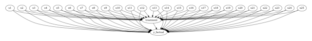
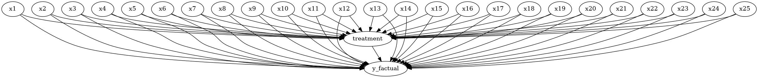
ihdp_model = CausalModel(
data=data,
treatment='treatment',
outcome='y_factual',
common_causes=common_causes
)
ihdp_model.view_model(layout="dot")
from IPython.display import Image, display
display(Image(filename="causal_model.png"))
Lalonde#
[5]:
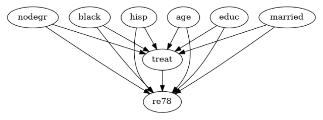
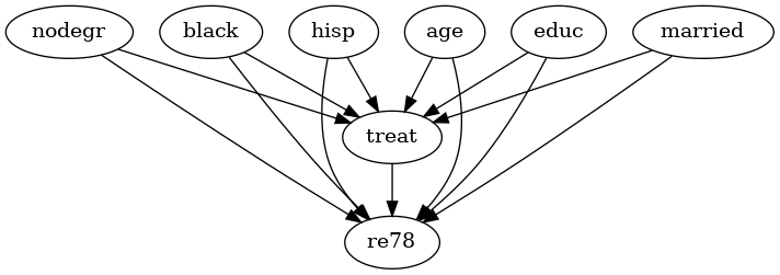
lalonde_model = CausalModel(
                data=lalonde,
                treatment='treat',
                outcome='re78',
                common_causes='nodegr+black+hisp+age+educ+married'.split('+')
            )
lalonde_model.view_model(layout="dot")
from IPython.display import Image, display
display(Image(filename="causal_model.png"))
步骤 2:识别#
IHDP#
[6]:
#Identify the causal effect for the ihdp dataset
ihdp_identified_estimand = ihdp_model.identify_effect(proceed_when_unidentifiable=True)
print(ihdp_identified_estimand)
Estimand type: EstimandType.NONPARAMETRIC_ATE

### Estimand : 1
Estimand name: backdoor
Estimand expression:
     d                                                                         ↪
────────────(E[y_factual|x25,x21,x12,x6,x18,x3,x15,x16,x8,x4,x11,x2,x24,x17,x2 ↪
d[treatment]                                                                   ↪

↪
↪ 3,x7,x9,x5,x22,x13,x19,x1,x20,x10,x14])
↪
Estimand assumption 1, Unconfoundedness: If U→{treatment} and U→y_factual then P(y_factual|treatment,x25,x21,x12,x6,x18,x3,x15,x16,x8,x4,x11,x2,x24,x17,x23,x7,x9,x5,x22,x13,x19,x1,x20,x10,x14,U) = P(y_factual|treatment,x25,x21,x12,x6,x18,x3,x15,x16,x8,x4,x11,x2,x24,x17,x23,x7,x9,x5,x22,x13,x19,x1,x20,x10,x14)

### Estimand : 2
Estimand name: iv
No such variable(s) found!

### Estimand : 3
Estimand name: frontdoor
No such variable(s) found!
Lalonde#
[7]:
#Identify the causal effect for the lalonde dataset
lalonde_identified_estimand = lalonde_model.identify_effect(proceed_when_unidentifiable=True)
print(lalonde_identified_estimand)
Estimand type: EstimandType.NONPARAMETRIC_ATE

### Estimand : 1
Estimand name: backdoor
Estimand expression:
   d
────────(E[re78|age,nodegr,educ,married,black,hisp])
d[treat]
Estimand assumption 1, Unconfoundedness: If U→{treat} and U→re78 then P(re78|treat,age,nodegr,educ,married,black,hisp,U) = P(re78|treat,age,nodegr,educ,married,black,hisp)

### Estimand : 2
Estimand name: iv
No such variable(s) found!

### Estimand : 3
Estimand name: frontdoor
No such variable(s) found!
步骤 3:估计 (使用倾向评分加权)#
IHDP#
[8]:
ihdp_estimate = ihdp_model.estimate_effect(
                    ihdp_identified_estimand,
                    method_name="backdoor.propensity_score_weighting"
                )

print("The Causal Estimate is " + str(ihdp_estimate.value))
The Causal Estimate is 4.028748218389962
Lalonde#
[9]:
lalonde_estimate = lalonde_model.estimate_effect(
                        lalonde_identified_estimand,
                        method_name="backdoor.propensity_score_weighting"
                    )

print("The Causal Estimate is " + str(lalonde_estimate.value))
The Causal Estimate is 1639.8089610946918
步骤 4:反驳#
IHDP#
添加随机共同原因#
[10]:
ihdp_refute_random_common_cause = ihdp_model.refute_estimate(
                                        ihdp_identified_estimand,
                                        ihdp_estimate,
                                        method_name="random_common_cause"
                                    )

print(ihdp_refute_random_common_cause)
Refute: Add a random common cause
Estimated effect:4.028748218389962
New effect:4.028748218389964
p value:1.0
用安慰剂替换治疗#
[11]:
ihdp_refute_placebo_treatment = ihdp_model.refute_estimate(
                                    ihdp_identified_estimand,
                                    ihdp_estimate,
                                    method_name="placebo_treatment_refuter",
                                    placebo_type="permute"
                                )

print(ihdp_refute_placebo_treatment)
Refute: Use a Placebo Treatment
Estimated effect:4.028748218389962
New effect:-0.4415444471465237
p value:0.02
移除随机数据子集#
[12]:
ihdp_refute_random_subset = ihdp_model.refute_estimate(
                                    ihdp_identified_estimand,
                                    ihdp_estimate,
                                    method_name="data_subset_refuter",
                                    subset_fraction=0.8
                            )
print(ihdp_refute_random_subset)
Refute: Use a subset of data
Estimated effect:4.028748218389962
New effect:4.03306148112277
p value:0.96
Lalonde#
添加随机共同原因#
[13]:
lalonde_refute_random_common_cause = lalonde_model.refute_estimate(
                                            lalonde_identified_estimand,
                                            lalonde_estimate,
                                            method_name="random_common_cause"
                                        )

print(lalonde_refute_random_common_cause)
Refute: Add a random common cause
Estimated effect:1639.8089610946918
New effect:1639.8089610946924
p value:1.0
用安慰剂替换治疗#
[14]:
lalonde_refute_placebo_treatment = lalonde_model.refute_estimate(
                                        lalonde_identified_estimand,
                                        lalonde_estimate,
                                        method_name="placebo_treatment_refuter",
                                        placebo_type="permute"
                                    )

print(lalonde_refute_placebo_treatment)
Refute: Use a Placebo Treatment
Estimated effect:1639.8089610946918
New effect:-156.25759930326174
p value:0.82
移除随机数据子集#
[15]:
lalonde_refute_random_subset = lalonde_model.refute_estimate(
                                    lalonde_identified_estimand,
                                    lalonde_estimate,
                                    method_name="data_subset_refuter",
                                    subset_fraction=0.9
                                )

print(lalonde_refute_random_subset)
Refute: Use a subset of data
Estimated effect:1639.8089610946918
New effect:1656.1546989508256
p value:0.8600000000000001