DoWhy:因果推断的不同估计方法#
这是 DoWhy 因果推断库的快速介绍。我们将加载一个样本数据集,并使用不同的方法来估计(预先指定的)治疗变量对(预先指定的)结果变量的因果效应。
我们将看到并非所有估计器都能为此数据集返回正确的效应。
首先,让我们添加 Python 查找 DoWhy 代码所需的路径并加载所有必需的软件包
[1]:
%load_ext autoreload
%autoreload 2
[2]:
import numpy as np
import pandas as pd
import logging

import dowhy
from dowhy import CausalModel
import dowhy.datasets
现在,让我们加载一个数据集。为简单起见,我们模拟一个数据集,其中公共原因与治疗之间、以及公共原因与结果之间存在线性关系。
Beta 是真实的因果效应。
[3]:
data = dowhy.datasets.linear_dataset(beta=10,
        num_common_causes=5,
        num_instruments = 2,
        num_treatments=1,
        num_samples=10000,
        treatment_is_binary=True,
        outcome_is_binary=False,
        stddev_treatment_noise=10)
df = data["df"]
df
[3]:
| Z0 | Z1 | W0 | W1 | W2 | W3 | W4 | v0 | y | |
|---|---|---|---|---|---|---|---|---|---|
| 0 | 1.0 | 0.479477 | 0.477095 | 1.132642 | 0.108390 | 0.382815 | 0.532607 | True | 14.968331 |
| 1 | 1.0 | 0.989410 | 0.915693 | -1.342175 | 0.670553 | 1.005776 | 0.332877 | True | 19.876419 |
| 2 | 1.0 | 0.820212 | -0.413122 | -2.197523 | 0.294065 | 0.852834 | 0.115160 | True | 13.483019 |
| 3 | 1.0 | 0.954148 | 0.035852 | -1.827038 | 0.424961 | -0.527072 | -0.605727 | True | 7.464827 |
| 4 | 1.0 | 0.203695 | 2.714909 | 0.470942 | -0.773594 | 0.723341 | -1.306709 | True | 14.276015 |
| ... | ... | ... | ... | ... | ... | ... | ... | ... | ... |
| 9995 | 1.0 | 0.611374 | 0.098375 | -0.625154 | 2.163267 | -0.021415 | -0.974123 | True | 18.078720 |
| 9996 | 1.0 | 0.823602 | -0.369129 | 0.792496 | 0.019248 | -0.193196 | 0.128058 | True | 8.958994 |
| 9997 | 1.0 | 0.893659 | -0.266886 | 1.225691 | -0.968349 | -0.255394 | -1.084577 | True | 2.566665 |
| 9998 | 1.0 | 0.835925 | 1.396273 | -1.301292 | -0.656232 | -0.634653 | 0.869848 | True | 7.887862 |
| 9999 | 1.0 | 0.776103 | -0.582994 | -0.607181 | 1.849334 | 1.112603 | -2.315254 | True | 18.291335 |
10000 行 × 9 列
请注意,我们正在使用 pandas dataframe 加载数据。
识别因果可估量#
现在我们以 DOT 图格式输入一个因果图。
[4]:
# With graph
model=CausalModel(
        data = df,
        treatment=data["treatment_name"],
        outcome=data["outcome_name"],
        graph=data["gml_graph"],
        instruments=data["instrument_names"]
        )
[5]:
model.view_model()
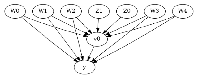
[6]:
from IPython.display import Image, display
display(Image(filename="causal_model.png"))
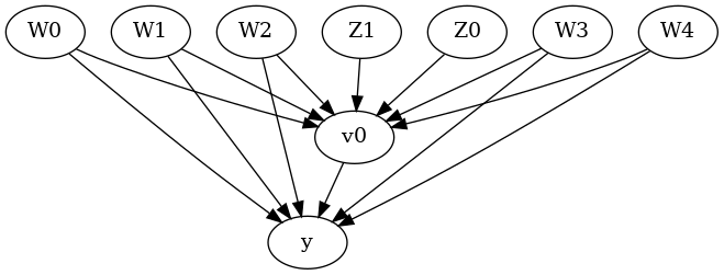
我们得到一个因果图。现在识别和估计已完成。
[7]:
identified_estimand = model.identify_effect(proceed_when_unidentifiable=True)
print(identified_estimand)
Estimand type: EstimandType.NONPARAMETRIC_ATE

### Estimand : 1
Estimand name: backdoor
Estimand expression:
  d
─────(E[y|W3,W0,W4,W2,W1])
d[v₀]
Estimand assumption 1, Unconfoundedness: If U→{v0} and U→y then P(y|v0,W3,W0,W4,W2,W1,U) = P(y|v0,W3,W0,W4,W2,W1)

### Estimand : 2
Estimand name: iv
Estimand expression:
 ⎡                              -1⎤
 ⎢    d        ⎛    d          ⎞  ⎥
E⎢─────────(y)⋅⎜─────────([v₀])⎟  ⎥
 ⎣d[Z₀  Z₁]    ⎝d[Z₀  Z₁]      ⎠  ⎦
Estimand assumption 1, As-if-random: If U→→y then ¬(U →→{Z0,Z1})
Estimand assumption 2, Exclusion: If we remove {Z0,Z1}→{v0}, then ¬({Z0,Z1}→y)

### Estimand : 3
Estimand name: frontdoor
No such variable(s) found!
方法 1:回归#
使用线性回归。
[8]:
causal_estimate_reg = model.estimate_effect(identified_estimand,
        method_name="backdoor.linear_regression",
        test_significance=True)
print(causal_estimate_reg)
print("Causal Estimate is " + str(causal_estimate_reg.value))
*** Causal Estimate ***

## Identified estimand
Estimand type: EstimandType.NONPARAMETRIC_ATE

### Estimand : 1
Estimand name: backdoor
Estimand expression:
  d
─────(E[y|W3,W0,W4,W2,W1])
d[v₀]
Estimand assumption 1, Unconfoundedness: If U→{v0} and U→y then P(y|v0,W3,W0,W4,W2,W1,U) = P(y|v0,W3,W0,W4,W2,W1)

## Realized estimand
b: y~v0+W3+W0+W4+W2+W1
Target units: ate

## Estimate
Mean value: 9.999731332644417
p-value: [0.]

Causal Estimate is 9.999731332644417
方法 2:距离匹配#
定义一个距离度量,然后使用该度量匹配治疗组和对照组之间最接近的点。
[9]:
causal_estimate_dmatch = model.estimate_effect(identified_estimand,
                                              method_name="backdoor.distance_matching",
                                              target_units="att",
                                              method_params={'distance_metric':"minkowski", 'p':2})
print(causal_estimate_dmatch)
print("Causal Estimate is " + str(causal_estimate_dmatch.value))
*** Causal Estimate ***

## Identified estimand
Estimand type: EstimandType.NONPARAMETRIC_ATE

### Estimand : 1
Estimand name: backdoor
Estimand expression:
  d
─────(E[y|W3,W0,W4,W2,W1])
d[v₀]
Estimand assumption 1, Unconfoundedness: If U→{v0} and U→y then P(y|v0,W3,W0,W4,W2,W1,U) = P(y|v0,W3,W0,W4,W2,W1)

## Realized estimand
b: y~v0+W3+W0+W4+W2+W1
Target units: att

## Estimate
Mean value: 11.278546846122476

Causal Estimate is 11.278546846122476
方法 3:倾向得分分层#
我们将使用倾向得分对数据中的单位进行分层。
[10]:
causal_estimate_strat = model.estimate_effect(identified_estimand,
                                              method_name="backdoor.propensity_score_stratification",
                                              target_units="att")
print(causal_estimate_strat)
print("Causal Estimate is " + str(causal_estimate_strat.value))
*** Causal Estimate ***

## Identified estimand
Estimand type: EstimandType.NONPARAMETRIC_ATE

### Estimand : 1
Estimand name: backdoor
Estimand expression:
  d
─────(E[y|W3,W0,W4,W2,W1])
d[v₀]
Estimand assumption 1, Unconfoundedness: If U→{v0} and U→y then P(y|v0,W3,W0,W4,W2,W1,U) = P(y|v0,W3,W0,W4,W2,W1)

## Realized estimand
b: y~v0+W3+W0+W4+W2+W1
Target units: att

## Estimate
Mean value: 9.932208243866834

Causal Estimate is 9.932208243866834
方法 4:倾向得分匹配#
我们将使用倾向得分对数据中的单位进行匹配。
[11]:
causal_estimate_match = model.estimate_effect(identified_estimand,
                                              method_name="backdoor.propensity_score_matching",
                                              target_units="atc")
print(causal_estimate_match)
print("Causal Estimate is " + str(causal_estimate_match.value))
*** Causal Estimate ***

## Identified estimand
Estimand type: EstimandType.NONPARAMETRIC_ATE

### Estimand : 1
Estimand name: backdoor
Estimand expression:
  d
─────(E[y|W3,W0,W4,W2,W1])
d[v₀]
Estimand assumption 1, Unconfoundedness: If U→{v0} and U→y then P(y|v0,W3,W0,W4,W2,W1,U) = P(y|v0,W3,W0,W4,W2,W1)

## Realized estimand
b: y~v0+W3+W0+W4+W2+W1
Target units: atc

## Estimate
Mean value: 9.643378784620955

Causal Estimate is 9.643378784620955
方法 5:加权#
我们将使用(逆)倾向得分对数据中的单位进行加权。DoWhy 支持几种不同的加权方案:1. 香草逆倾向得分加权 (IPS) (weighting_scheme=”ips_weight”) 2. 自归一化 IPS 加权(也称为 Hajek 估计器)(weighting_scheme=”ips_normalized_weight”) 3. 稳定化 IPS 加权 (weighting_scheme = “ips_stabilized_weight”)
[12]:
causal_estimate_ipw = model.estimate_effect(identified_estimand,
                                            method_name="backdoor.propensity_score_weighting",
                                            target_units = "ate",
                                            method_params={"weighting_scheme":"ips_weight"})
print(causal_estimate_ipw)
print("Causal Estimate is " + str(causal_estimate_ipw.value))
*** Causal Estimate ***

## Identified estimand
Estimand type: EstimandType.NONPARAMETRIC_ATE

### Estimand : 1
Estimand name: backdoor
Estimand expression:
  d
─────(E[y|W3,W0,W4,W2,W1])
d[v₀]
Estimand assumption 1, Unconfoundedness: If U→{v0} and U→y then P(y|v0,W3,W0,W4,W2,W1,U) = P(y|v0,W3,W0,W4,W2,W1)

## Realized estimand
b: y~v0+W3+W0+W4+W2+W1
Target units: ate

## Estimate
Mean value: 12.478466888961442

Causal Estimate is 12.478466888961442
方法 6:工具变量#
我们将使用提供的工具变量的 Wald 估计器。
[13]:
causal_estimate_iv = model.estimate_effect(identified_estimand,
        method_name="iv.instrumental_variable", method_params = {'iv_instrument_name': 'Z0'})
print(causal_estimate_iv)
print("Causal Estimate is " + str(causal_estimate_iv.value))
*** Causal Estimate ***

## Identified estimand
Estimand type: EstimandType.NONPARAMETRIC_ATE

### Estimand : 1
Estimand name: iv
Estimand expression:
 ⎡                              -1⎤
 ⎢    d        ⎛    d          ⎞  ⎥
E⎢─────────(y)⋅⎜─────────([v₀])⎟  ⎥
 ⎣d[Z₀  Z₁]    ⎝d[Z₀  Z₁]      ⎠  ⎦
Estimand assumption 1, As-if-random: If U→→y then ¬(U →→{Z0,Z1})
Estimand assumption 2, Exclusion: If we remove {Z0,Z1}→{v0}, then ¬({Z0,Z1}→y)

## Realized estimand
Realized estimand: Wald Estimator
Realized estimand type: EstimandType.NONPARAMETRIC_ATE
Estimand expression:
 ⎡ d    ⎤
E⎢───(y)⎥
 ⎣dZ₀   ⎦
──────────
 ⎡ d     ⎤
E⎢───(v₀)⎥
 ⎣dZ₀    ⎦
Estimand assumption 1, As-if-random: If U→→y then ¬(U →→{Z0,Z1})
Estimand assumption 2, Exclusion: If we remove {Z0,Z1}→{v0}, then ¬({Z0,Z1}→y)
Estimand assumption 3, treatment_effect_homogeneity: Each unit's treatment ['v0'] is affected in the same way by common causes of ['v0'] and ['y']
Estimand assumption 4, outcome_effect_homogeneity: Each unit's outcome ['y'] is affected in the same way by common causes of ['v0'] and ['y']

Target units: ate

## Estimate
Mean value: 7.667844609940294

Causal Estimate is 7.667844609940294
方法 7:回归不连续性#
我们将在内部将其转换为等效的工具变量问题。
[14]:
causal_estimate_regdist = model.estimate_effect(identified_estimand,
        method_name="iv.regression_discontinuity",
        method_params={'rd_variable_name':'Z1',
                       'rd_threshold_value':0.5,
                       'rd_bandwidth': 0.15})
print(causal_estimate_regdist)
print("Causal Estimate is " + str(causal_estimate_regdist.value))
*** Causal Estimate ***

## Identified estimand
Estimand type: EstimandType.NONPARAMETRIC_ATE

### Estimand : 1
Estimand name: iv
Estimand expression:
 ⎡                              -1⎤
 ⎢    d        ⎛    d          ⎞  ⎥
E⎢─────────(y)⋅⎜─────────([v₀])⎟  ⎥
 ⎣d[Z₀  Z₁]    ⎝d[Z₀  Z₁]      ⎠  ⎦
Estimand assumption 1, As-if-random: If U→→y then ¬(U →→{Z0,Z1})
Estimand assumption 2, Exclusion: If we remove {Z0,Z1}→{v0}, then ¬({Z0,Z1}→y)

## Realized estimand
Realized estimand: Wald Estimator
Realized estimand type: EstimandType.NONPARAMETRIC_ATE
Estimand expression:
 ⎡        d            ⎤
E⎢──────────────────(y)⎥
 ⎣dlocal_rd_variable   ⎦
─────────────────────────
 ⎡        d             ⎤
E⎢──────────────────(v₀)⎥
 ⎣dlocal_rd_variable    ⎦
Estimand assumption 1, As-if-random: If U→→y then ¬(U →→{Z0,Z1})
Estimand assumption 2, Exclusion: If we remove {Z0,Z1}→{v0}, then ¬({Z0,Z1}→y)
Estimand assumption 3, treatment_effect_homogeneity: Each unit's treatment ['v0'] is affected in the same way by common causes of ['v0'] and ['y']
Estimand assumption 4, outcome_effect_homogeneity: Each unit's outcome ['y'] is affected in the same way by common causes of ['v0'] and ['y']

Target units: ate

## Estimate
Mean value: 4.226754677196832

Causal Estimate is 4.226754677196832