DoWhy 在 Lalonde 数据集上的示例

感谢 [@mizuy](mizuy) 提供此示例。这里我们使用 Lalonde 数据集并对其应用 IPW 估计器。

1. 加载数据

import dowhy.datasets

lalonde = dowhy.datasets.lalonde_dataset()

2. 运行 DoWhy 分析：建模、识别、估计

from dowhy import CausalModel


model=CausalModel(
        data = lalonde,
        treatment='treat',
        outcome='re78',
        common_causes='nodegr+black+hisp+age+educ+married'.split('+'))
identified_estimand = model.identify_effect(proceed_when_unidentifiable=True)
estimate = model.estimate_effect(identified_estimand,
        method_name="backdoor.propensity_score_weighting",
        target_units="ate",
        method_params={"weighting_scheme":"ips_weight"})

print("Causal Estimate is " + str(estimate.value))

import statsmodels.formula.api as smf
reg=smf.wls('re78~1+treat', data=lalonde, weights=lalonde.ips_stabilized_weight)
res=reg.fit()
res.summary()

Causal Estimate is 1639.8254852564396

WLS 回归结果

因变量	re78	R 方	0.015
模型	WLS	调整的 R 方	0.013
方法	最小二乘法	F 统计量	6.743
日期	Sun, 24 Nov 2024	Prob (F 统计量)	0.00972
时间	18:09:33	对数似然	-4544.7
观测数	445	AIC	9093.
残差自由度	443	BIC	9102.
模型自由度	1
协方差类型	非稳健

	系数	标准误	t 值	P>|t|	[0.025	0.975]
截距	4555.0717	406.705	11.200	0.000	3755.761	5354.383
treat[T.True]	1639.8255	631.496	2.597	0.010	398.725	2880.926

Omnibus	303.265	Durbin-Watson	2.085
Prob(Omnibus)	0.000	Jarque-Bera (JB)	4770.724
偏度	2.709	Prob(JB)	0.00
峰度	18.097	条件数	2.47

注释
[1] 标准误假定误差的协方差矩阵是正确指定的。

3. 解释估计结果

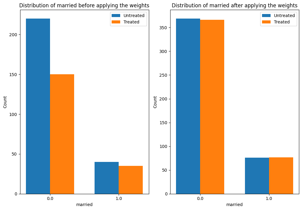
下图显示了混杂因素“已婚”的分布如何从原始数据变为加权数据。在这两个数据集中，我们比较了处理组和未处理组中“已婚”的分布。

estimate.interpret(method_name="confounder_distribution_interpreter",var_type='discrete',
                   var_name='married', fig_size = (10, 7), font_size = 12)

4. 检查合理性：与手动 IPW 估计结果进行比较

df = model._data
ps = df['propensity_score']
y = df['re78']
z = df['treat']

ey1 = z*y/ps / sum(z/ps)
ey0 = (1-z)*y/(1-ps) / sum((1-z)/(1-ps))
ate = ey1.sum()-ey0.sum()
print("Causal Estimate is " + str(ate))

# correct -> Causal Estimate is 1634.9868359746906

Causal Estimate is 1639.8254852564378