DoWhy 因果 API 演示

我们展示一个将因果扩展添加到任何数据框的简单示例。

import dowhy.datasets
import dowhy.api
from dowhy.graph import build_graph_from_str

import numpy as np
import pandas as pd

from statsmodels.api import OLS

data = dowhy.datasets.linear_dataset(beta=5,
        num_common_causes=1,
        num_instruments = 0,
        num_samples=1000,
        treatment_is_binary=True)
df = data['df']
df['y'] = df['y'] + np.random.normal(size=len(df)) # Adding noise to data. Without noise, the variance in Y|X, Z is zero, and mcmc fails.
nx_graph = build_graph_from_str(data["dot_graph"])

treatment= data["treatment_name"][0]
outcome = data["outcome_name"][0]
common_cause = data["common_causes_names"][0]
df

	W0	v0	y
0	0.037488	False	-0.174667
1	-0.523050	False	-1.292853
2	2.070420	True	9.443895
3	0.068183	False	1.113386
4	0.104074	True	5.843495
...	...	...	...
995	-0.265148	True	4.197523
996	-0.973204	False	-0.142424
997	-1.241690	False	-2.795862
998	-1.825721	False	-3.752621
999	-0.607617	True	2.775188

1000 行 × 3 列

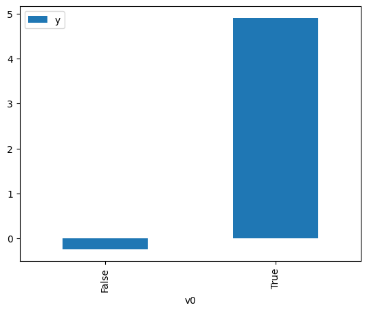
# data['df'] is just a regular pandas.DataFrame
df.causal.do(x=treatment,
             variable_types={treatment: 'b', outcome: 'c', common_cause: 'c'},
             outcome=outcome,
             common_causes=[common_cause],
            ).groupby(treatment).mean().plot(y=outcome, kind='bar')

<Axes: xlabel='v0'>

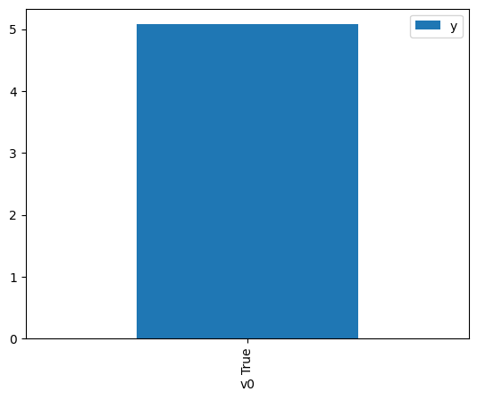
df.causal.do(x={treatment: 1},
              variable_types={treatment:'b', outcome: 'c', common_cause: 'c'},
              outcome=outcome,
              method='weighting',
              common_causes=[common_cause]
              ).groupby(treatment).mean().plot(y=outcome, kind='bar')

<Axes: xlabel='v0'>

cdf_1 = df.causal.do(x={treatment: 1},
              variable_types={treatment: 'b', outcome: 'c', common_cause: 'c'},
              outcome=outcome,
              graph=nx_graph
              )

cdf_0 = df.causal.do(x={treatment: 0},
              variable_types={treatment: 'b', outcome: 'c', common_cause: 'c'},
              outcome=outcome,
              graph=nx_graph
              )

cdf_0

	W0	v0	y	倾向得分	权重
0	-0.713942	False	-0.832839	0.774908	1.290476
1	0.378506	False	1.757012	0.329282	3.036907
2	-0.416285	False	-1.897409	0.669419	1.493834
3	-1.022786	False	-3.304443	0.856541	1.167486
4	0.541459	False	1.429673	0.268558	3.723594
...	...	...	...	...	...
995	-0.873678	False	0.280653	0.820688	1.218489
996	0.933586	False	2.296218	0.154328	6.479718
997	-0.961088	False	-1.653206	0.842488	1.186961
998	-0.057126	False	0.769879	0.516302	1.936850
999	-0.328091	False	0.223023	0.633746	1.577919

1000 行 × 5 列

cdf_1

	W0	v0	y	倾向得分	权重
0	-0.752117	True	3.312724	0.213443	4.685087
1	-0.568538	True	4.378100	0.273487	3.656476
2	1.378671	True	7.617855	0.923760	1.082532
3	0.917073	True	6.610054	0.841791	1.187943
4	-0.871327	True	2.153620	0.179929	5.557742
...	...	...	...	...	...
995	0.260021	True	5.172035	0.622504	1.606415
996	3.495361	True	14.133175	0.998108	1.001895
997	-1.526145	True	1.050194	0.063908	15.647445
998	-0.324753	True	4.160558	0.367636	2.720078
999	1.709055	True	6.392574	0.956211	1.045794

1000 行 × 5 列

将估计值与线性回归进行比较

首先，使用因果数据框估计效应，并计算 95% 置信区间。

(cdf_1['y'] - cdf_0['y']).mean()

$\displaystyle 5.40925954703069$

1.96*(cdf_1['y'] - cdf_0['y']).std() / np.sqrt(len(df))

$\displaystyle 0.191657653401046$

与 OLS 的估计值进行比较。

model = OLS(np.asarray(df[outcome]), np.asarray(df[[common_cause, treatment]], dtype=np.float64))
result = model.fit()
result.summary()

OLS 回归结果

因变量	y	R 方 (未中心化)	0.957
模型	OLS	调整 R 方 (未中心化)	0.957
方法	最小二乘法	F 统计量	1.102e+04
日期	Sun, 24 Nov 2024	概率 (F 统计量)	0.00
时间	18:03:52	对数似然	-1410.0
观测数量	1000	AIC	2824.
残差自由度	998	BIC	2834.
模型自由度	2
协方差类型	非稳健

	系数	标准误	t	P>|t|	[0.025	0.975]
x1	2.1425	0.034	63.535	0.000	2.076	2.209
x2	4.9804	0.048	103.470	0.000	4.886	5.075

Omnibus	0.734	Durbin-Watson	1.928
概率(Omnibus)	0.693	Jarque-Bera (JB)	0.658
偏度	0.060	概率(JB)	0.720
峰度	3.038	条件数	1.67

注释
[1] R² 是在未中心化的情况下计算的，因为模型不包含常数项。
[2] 标准误假设误差的协方差矩阵已正确指定。