查找微服务架构中延迟升高的根本原因#
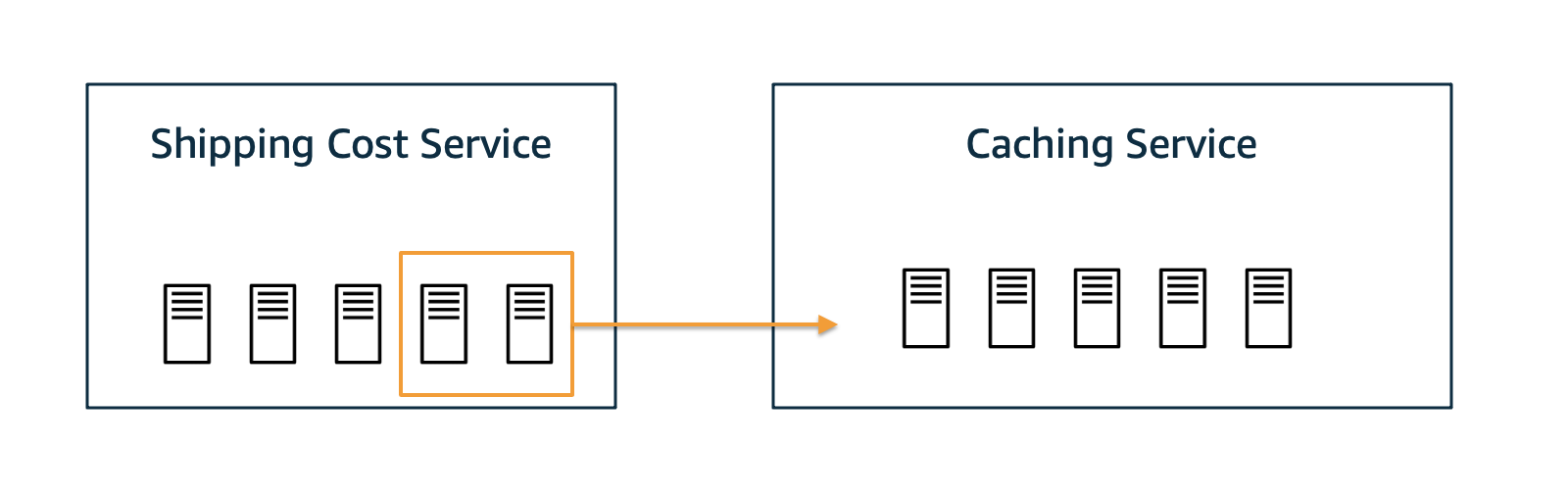
在本案例研究中,我们将找出支持在线商店的云服务中观察到的“意外”延迟的根本原因。我们专注于下单过程,该过程涉及不同的服务,以确保所下订单有效、客户经过身份验证、运费计算正确以及发货流程相应启动。服务之间的依赖关系如下图所示。
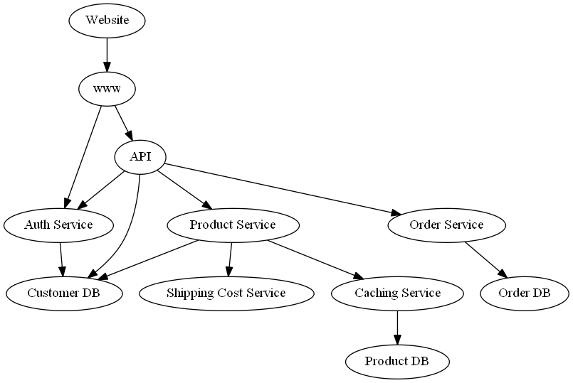
这种依赖关系图可以从 Amazon X-Ray 等服务获取,或者根据请求的跟踪结构手动定义。
我们假设上述依赖关系图是正确的,并且我们能够测量订单请求中每个节点的延迟(以秒为单位)。对于 Website,延迟代表显示订单确认之前的时间。为简单起见,我们假设服务是同步的,即服务必须等待下游服务才能继续进行。此外,我们假设两个节点不会同时受到未观测因素(隐藏混杂因素)的影响(即因果充足性)。考虑到例如网络流量会影响多个服务,这个假设在实际场景中可能会被违反。然而,弱混杂因素可以忽略不计,而强混杂因素(如网络流量)可能会错误地将多个节点视为根本原因。一般来说,我们只能识别数据中包含的原因。
在这些假设下,观测到的节点延迟由节点本身的延迟(固有延迟)和所有直接子节点延迟的总和决定。这也可能包括多次调用子节点的情况。
让我们加载包含每个节点观测延迟的数据。
[1]:
import pandas as pd

normal_data = pd.read_csv("rca_microservice_architecture_latencies.csv")
normal_data.head()
[1]:
| Product DB | Customer DB | Order DB | Shipping Cost Service | Caching Service | Product Service | Auth Service | Order Service | API | www | Website | |
|---|---|---|---|---|---|---|---|---|---|---|---|
| 0 | 0.553608 | 0.057729 | 0.153977 | 0.120217 | 0.122195 | 0.391738 | 0.399664 | 0.710525 | 2.103962 | 2.580403 | 2.971071 |
| 1 | 0.053393 | 0.239560 | 0.297794 | 0.142854 | 0.275471 | 0.545372 | 0.646370 | 0.991620 | 2.932192 | 3.804571 | 3.895535 |
| 2 | 0.023860 | 0.300044 | 0.042169 | 0.125017 | 0.152685 | 0.574918 | 0.672228 | 0.964807 | 3.106218 | 4.076227 | 4.441924 |
| 3 | 0.118598 | 0.478097 | 0.042383 | 0.143969 | 0.222720 | 0.618129 | 0.638179 | 0.938366 | 3.217643 | 4.043560 | 4.334924 |
| 4 | 0.524901 | 0.078031 | 0.031694 | 0.231884 | 0.647452 | 1.081753 | 0.388506 | 0.711937 | 2.793605 | 3.215307 | 3.255062 |
我们再来看一下变量的成对散点图和直方图。
[2]:
axes = pd.plotting.scatter_matrix(normal_data, figsize=(10, 10), c='#ff0d57', alpha=0.2, hist_kwds={'color':['#1E88E5']});
for ax in axes.flatten():
    ax.xaxis.label.set_rotation(90)
    ax.yaxis.label.set_rotation(0)
    ax.yaxis.label.set_ha('right')
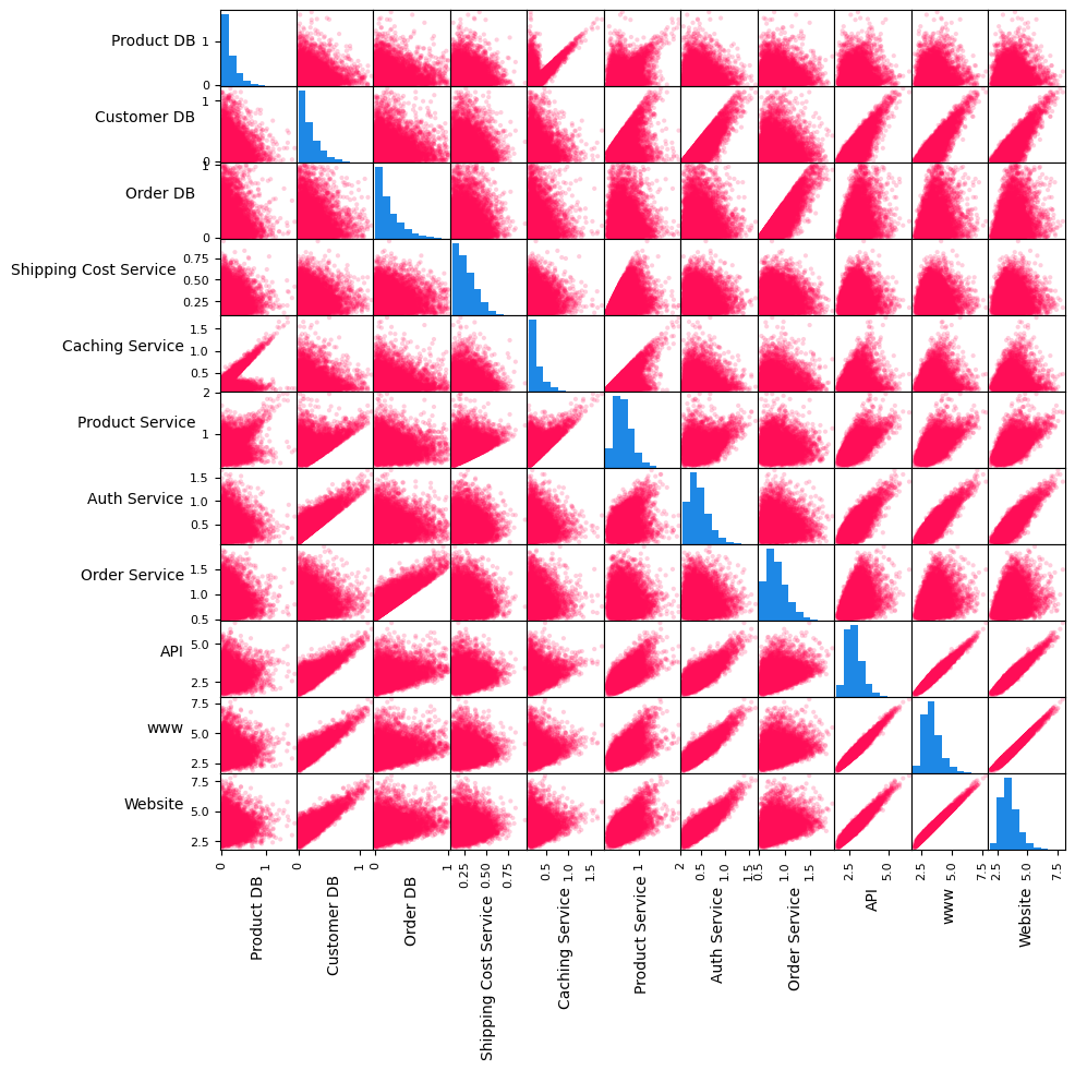
在上面的矩阵中,对角线上的图是变量的直方图,而对角线外的图是变量对的散点图。没有依赖关系的服务(即 Customer DB、Product DB、Order DB 和 Shipping Cost Service)的直方图形状类似于高斯分布的一半。各种变量对(例如 API 和 www、www 和 Website、Order Service 和 Order DB)的散点图显示出线性关系。我们很快就会利用这些信息为因果图中的节点分配生成因果模型。
设置因果模型#
如果我们看 Website 节点,很明显我们在此处经历的延迟取决于所有下游节点的延迟。特别是,如果一个下游节点耗时很长,Website 显示更新也需要很长时间。由此可见,可以通过反转服务图的箭头来构建延迟的因果图。
[3]:
import networkx as nx
from dowhy import gcm
from dowhy.utils import plot, bar_plot
gcm.util.general.set_random_seed(0)

causal_graph = nx.DiGraph([('www', 'Website'),
                           ('Auth Service', 'www'),
                           ('API', 'www'),
                           ('Customer DB', 'Auth Service'),
                           ('Customer DB', 'API'),
                           ('Product Service', 'API'),
                           ('Auth Service', 'API'),
                           ('Order Service', 'API'),
                           ('Shipping Cost Service', 'Product Service'),
                           ('Caching Service', 'Product Service'),
                           ('Product DB', 'Caching Service'),
                           ('Customer DB', 'Product Service'),
                           ('Order DB', 'Order Service')])
[4]:
plot(causal_graph, figure_size=[13, 13])
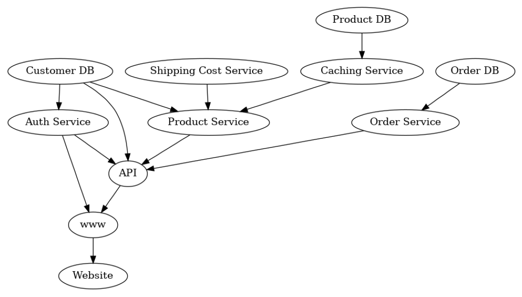
在这里,我们感兴趣的是服务延迟之间的因果关系,而不是调用服务的顺序。
我们将利用成对散点图和直方图中的信息手动分配因果模型。特别是,我们将半正态分布分配给根节点(即 Customer DB、Product DB、Order DB 和 Shipping Cost Service)。对于非根节点,我们分配线性加性噪声模型(许多父子对的散点图表明如此),并使用噪声项的经验分布。
[5]:
from scipy.stats import halfnorm

causal_model = gcm.StructuralCausalModel(causal_graph)

for node in causal_graph.nodes:
    if len(list(causal_graph.predecessors(node))) > 0:
        causal_model.set_causal_mechanism(node, gcm.AdditiveNoiseModel(gcm.ml.create_linear_regressor()))
    else:
        causal_model.set_causal_mechanism(node, gcm.ScipyDistribution(halfnorm))
或者,如果我们在没有先验知识或不熟悉统计含义的情况下,也可以自动化此过程。
gcm.auto.assign_causal_mechanisms(causal_model, normal_data)
在继续第一个场景之前,让我们先评估一下我们的因果模型
[6]:
gcm.fit(causal_model, normal_data)
print(gcm.evaluate_causal_model(causal_model, normal_data))
Fitting causal mechanism of node Order DB: 100%|██████████| 11/11 [00:00<00:00, 74.45it/s]
Evaluating causal mechanisms...: 100%|██████████| 11/11 [00:02<00:00,  4.57it/s]
Test permutations of given graph: 100%|██████████| 50/50 [01:13<00:00,  1.47s/it]
Evaluated the performance of the causal mechanisms and the invertibility assumption of the causal mechanisms and the overall average KL divergence between generated and observed distribution and the graph structure. The results are as follows:
==== Evaluation of Causal Mechanisms ====
The used evaluation metrics are:
- KL divergence (only for root-nodes): Evaluates the divergence between the generated and the observed distribution.
- Mean Squared Error (MSE): Evaluates the average squared differences between the observed values and the conditional expectation of the causal mechanisms.
- Normalized MSE (NMSE): The MSE normalized by the standard deviation for better comparison.
- R2 coefficient: Indicates how much variance is explained by the conditional expectations of the mechanisms. Note, however, that this can be misleading for nonlinear relationships.
- F1 score (only for categorical non-root nodes): The harmonic mean of the precision and recall indicating the goodness of the underlying classifier model.
- (normalized) Continuous Ranked Probability Score (CRPS): The CRPS generalizes the Mean Absolute Percentage Error to probabilistic predictions. This gives insights into the accuracy and calibration of the causal mechanisms.
NOTE: Every metric focuses on different aspects and they might not consistently indicate a good or bad performance.
We will mostly utilize the CRPS for comparing and interpreting the performance of the mechanisms, since this captures the most important properties for the causal model.
--- Node Customer DB
- The KL divergence between generated and observed distribution is 0.026730847930932323.
The estimated KL divergence indicates an overall very good representation of the data distribution.
--- Node Shipping Cost Service
- The KL divergence between generated and observed distribution is 0.0.
The estimated KL divergence indicates an overall very good representation of the data distribution.
--- Node Product DB
- The KL divergence between generated and observed distribution is 0.04309162176082666.
The estimated KL divergence indicates an overall very good representation of the data distribution.
--- Node Order DB
- The KL divergence between generated and observed distribution is 0.03223241982914243.
The estimated KL divergence indicates an overall very good representation of the data distribution.
--- Node Auth Service
- The MSE is 0.014405407564615797.
- The NMSE is 0.5465495860903358.
- The R2 coefficient is 0.7012359660103364.
- The normalized CRPS is 0.30265499391971407.
The estimated CRPS indicates a good model performance.
--- Node Caching Service
- The MSE is 0.02313410655739081.
- The NMSE is 0.8421286359832795.
- The R2 coefficient is 0.2907975654579837.
- The normalized CRPS is 0.46264654494762336.
The estimated CRPS indicates only a fair model performance. Note, however, that a high CRPS could also result from a small signal to noise ratio.
--- Node Order Service
- The MSE is 0.014402623661901339.
- The NMSE is 0.5485279868056235.
- The R2 coefficient is 0.6990119423108653.
- The normalized CRPS is 0.30321497413904863.
The estimated CRPS indicates a good model performance.
--- Node Product Service
- The MSE is 0.020441295317239063.
- The NMSE is 0.6498526098564431.
- The R2 coefficient is 0.5775517273698512.
- The normalized CRPS is 0.3643692225262228.
The estimated CRPS indicates only a fair model performance. Note, however, that a high CRPS could also result from a small signal to noise ratio.
--- Node API
- The MSE is 0.014478740667166996.
- The NMSE is 0.20970446018379812.
- The R2 coefficient is 0.9559977978951697.
- The normalized CRPS is 0.11586910197147379.
The estimated CRPS indicates a very good model performance.
--- Node www
- The MSE is 0.011040360284322542.
- The NMSE is 0.1375983208617472.
- The R2 coefficient is 0.9810608560286648.
- The normalized CRPS is 0.0779437689368548.
The estimated CRPS indicates a very good model performance.
--- Node Website
- The MSE is 0.020774228074041143.
- The NMSE is 0.185120350663801.
- The R2 coefficient is 0.9657171988034176.
- The normalized CRPS is 0.10227892839479753.
The estimated CRPS indicates a very good model performance.
==== Evaluation of Invertible Functional Causal Model Assumption ====
--- The model assumption for node www is not rejected with a p-value of 1.0 (after potential adjustment) and a significance level of 0.05.
This implies that the model assumption might be valid.
--- The model assumption for node Website is not rejected with a p-value of 1.0 (after potential adjustment) and a significance level of 0.05.
This implies that the model assumption might be valid.
--- The model assumption for node Auth Service is not rejected with a p-value of 0.46642517211292034 (after potential adjustment) and a significance level of 0.05.
This implies that the model assumption might be valid.
--- The model assumption for node API is rejected with a p-value of 0.010732197989039571 (after potential adjustment) and a significance level of 0.05.
This implies that the model assumption might not be valid. This is, the relationship cannot be represent with this type of mechanism or there is a hidden confounder between the node and its parents.
--- The model assumption for node Product Service is rejected with a p-value of 0.0 (after potential adjustment) and a significance level of 0.05.
This implies that the model assumption might not be valid. This is, the relationship cannot be represent with this type of mechanism or there is a hidden confounder between the node and its parents.
--- The model assumption for node Order Service is not rejected with a p-value of 1.0 (after potential adjustment) and a significance level of 0.05.
This implies that the model assumption might be valid.
--- The model assumption for node Caching Service is rejected with a p-value of 0.0 (after potential adjustment) and a significance level of 0.05.
This implies that the model assumption might not be valid. This is, the relationship cannot be represent with this type of mechanism or there is a hidden confounder between the node and its parents.
Note that these results are based on statistical independence tests, and the fact that the assumption was not rejected does not necessarily imply that it is correct. There is just no evidence against it.
==== Evaluation of Generated Distribution ====
The overall average KL divergence between the generated and observed distribution is 0.11748736081286179
The estimated KL divergence indicates an overall very good representation of the data distribution.
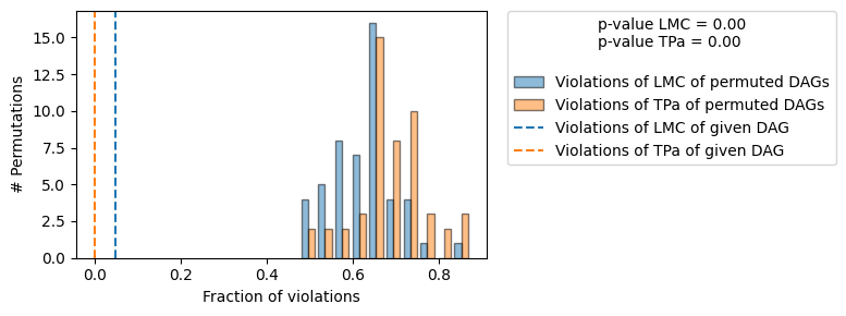
==== Evaluation of the Causal Graph Structure ====
+-------------------------------------------------------------------------------------------------------+
| Falsification Summary |
+-------------------------------------------------------------------------------------------------------+
| The given DAG is informative because 0 / 50 of the permutations lie in the Markov |
| equivalence class of the given DAG (p-value: 0.00). |
| The given DAG violates 3/63 LMCs and is better than 100.0% of the permuted DAGs (p-value: 0.00). |
| Based on the provided significance level (0.2) and because the DAG is informative, |
| we do not reject the DAG. |
+-------------------------------------------------------------------------------------------------------+
==== NOTE ====
Always double check the made model assumptions with respect to the graph structure and choice of causal mechanisms.
All these evaluations give some insight into the goodness of the causal model, but should not be overinterpreted, since some causal relationships can be intrinsically hard to model. Furthermore, many algorithms are fairly robust against misspecifications or poor performances of causal mechanisms.
这证实了我们因果模型的良好性。然而,我们也看到对于两个节点('Product Service' 和 'Caching Service'),加性噪声模型假设被违反了。这也与数据生成过程一致,其中这两个节点遵循非加性噪声模型。正如我们在下文中所见,大多数算法对于这种违反或因果机制的性能不佳仍然相当鲁棒。
要获得更详细的见解,请将 compare_mechanism_baselines 设置为 True。但这会花费更长时间。
场景 1:观测单个异常值#
假设我们的系统发出了警报,一位客户在下单时经历了异常高的延迟。我们现在的任务是调查这个问题并找出这种行为的根本原因。
我们首先加载与相应警报关联的延迟数据。
[7]:
outlier_data = pd.read_csv("rca_microservice_architecture_anomaly.csv")
outlier_data
[7]:
| Product DB | Customer DB | Order DB | Shipping Cost Service | Caching Service | Product Service | Auth Service | Order Service | API | www | Website | |
|---|---|---|---|---|---|---|---|---|---|---|---|
| 0 | 0.493145 | 0.180896 | 0.192593 | 0.197001 | 2.130865 | 2.48584 | 0.533847 | 1.132151 | 4.85583 | 5.522179 | 5.572588 |
我们关注客户直接体验到的 Website 延迟增加。
[8]:
outlier_data.iloc[0]['Website']-normal_data['Website'].mean()
[8]:
对于这位客户,Website 平均比其他客户慢了大约 2 秒。为什么会这样?
将目标服务的异常延迟归因于其他服务#
为了回答为什么 Website 对于这位客户来说较慢,我们将 Website 的异常延迟归因于因果图中的上游服务。有关此 API 背后的科学细节,请参阅 Janzing et al., 2019。我们将计算我们归因的 95% 自助法置信区间。特别是,我们从正常数据的随机子集中学习因果模型,并使用这些模型归因目标异常值分数,重复此过程 10 次。这样,我们报告的置信区间考虑了 (a) 我们因果模型的不确定性以及 (b) 由于从这些因果模型中抽取的样本方差导致的归因不确定性。
[9]:
gcm.config.disable_progress_bars() # to disable print statements when computing Shapley values

median_attribs, uncertainty_attribs = gcm.confidence_intervals(
    gcm.fit_and_compute(gcm.attribute_anomalies,
                        causal_model,
                        normal_data,
                        target_node='Website',
                        anomaly_samples=outlier_data),
    num_bootstrap_resamples=10)
默认情况下,使用基于分位数的异常分数,该分数估计样本正常的负对数概率。也就是说,异常值概率越高,分数越大。该库提供了不同类型的异常值评分函数,例如 z 分数,其中均值是基于因果模型的期望值。
让我们用条形图可视化归因及其不确定性。
[10]:
bar_plot(median_attribs, uncertainty_attribs, 'Attribution Score')
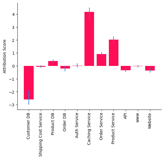
归因结果表明,Caching Service 是 Website 高延迟的主要驱动因素,这在意料之中,因为我们扰动了 Caching Service 的因果机制,从而在 Website 中产生了异常延迟(参见下面的附录)。有趣的是,Customer DB 有负贡献,表明它特别快,降低了 Website 中的异常值。请注意,有些归因也可能是由于模型错误指定造成的。例如,Caching Service 和 Product DB 之间的父子关系似乎表明存在两种机制。这可能是由于一个未观测的二元变量(例如,缓存命中/未命中)对 Caching Service 产生了乘性效应。加性噪声无法捕捉这个未观测变量的乘性效应。
场景 2:观测延迟永久性退化#
在之前的场景中,我们将 Website 中的一个单个异常延迟归因于因果图中的节点服务,这对于进行个别深入分析很有用。接下来,我们考虑一个场景,我们观察到延迟的永久性退化,并希望了解其驱动因素。特别是,我们将 Website 平均延迟的变化归因于上游节点。
假设我们额外收到 1000 个延迟更高的请求,如下所示。
[11]:
outlier_data = pd.read_csv("rca_microservice_architecture_anomaly_1000.csv")
outlier_data.head()
[11]:
| Product DB | Customer DB | Order DB | Shipping Cost Service | Caching Service | Product Service | Auth Service | Order Service | API | www | Website | |
|---|---|---|---|---|---|---|---|---|---|---|---|
| 0 | 0.140874 | 0.270117 | 0.021619 | 0.159421 | 2.201327 | 2.453859 | 0.958687 | 0.572128 | 4.921074 | 5.891927 | 5.937950 |
| 1 | 0.160903 | 0.008235 | 0.182182 | 0.114568 | 2.105901 | 2.259432 | 0.325054 | 0.683030 | 4.009969 | 4.373290 | 4.418746 |
| 2 | 0.013300 | 0.127177 | 0.591904 | 0.112362 | 2.160395 | 2.278189 | 0.645109 | 1.097460 | 4.915487 | 5.578015 | 5.708616 |
| 3 | 1.317167 | 0.145850 | 0.094301 | 0.401206 | 3.505417 | 3.622197 | 0.502680 | 0.880008 | 5.652773 | 6.265665 | 6.356730 |
| 4 | 0.699519 | 0.425039 | 0.233269 | 0.572897 | 2.931482 | 3.062255 | 0.598265 | 0.885846 | 5.585744 | 6.266662 | 6.346390 |
我们关注客户直接体验到的 1000 个请求的 Website 平均延迟增加。
[12]:
outlier_data['Website'].mean() - normal_data['Website'].mean()
[12]:
Website 平均比平时慢(几乎慢了 2 秒)。为什么会这样?
将目标服务的永久性延迟退化归因于其他服务#
为了回答为什么对于这 1000 个请求,Website 比之前慢,我们将 Website 平均延迟的变化归因于因果图中的上游服务。有关此 API 背后的科学细节,请参阅 Budhathoki et al., 2021。与之前的场景一样,我们将计算我们归因的 95% 自助法置信区间,并将其可视化为条形图。
[13]:
import numpy as np

median_attribs, uncertainty_attribs = gcm.confidence_intervals(
    lambda : gcm.distribution_change(causal_model,
                                     normal_data.sample(frac=0.6),
                                     outlier_data.sample(frac=0.6),
                                     'Website',
                                     difference_estimation_func=lambda x, y: np.mean(y) - np.mean(x)),
    num_bootstrap_resamples = 10)

bar_plot(median_attribs, uncertainty_attribs, 'Attribution Score')
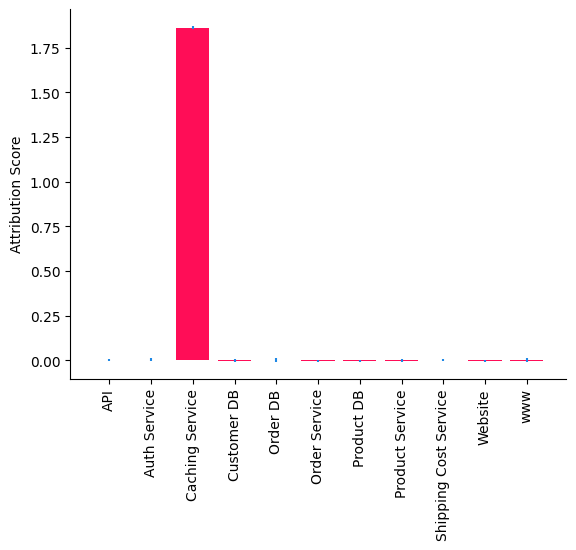
我们观察到 Caching Service 是导致 Website 变慢的根本原因。特别是,我们使用的方法告诉我们,Caching Service 的因果机制(即输入-输出行为)发生变化(例如,缓存算法)导致 Website 变慢。这也符合预期,因为异常延迟是通过改变 Caching Service 的因果机制生成的(参见下面的附录)。
场景 3:模拟资源转移的干预#
接下来,让我们想象一个场景,其中发生了场景 2 中的永久性退化,并且我们成功地将 Caching Service 识别为根本原因。此外,我们发现 Caching Service 的最近一次部署包含一个导致主机过载的错误。必须部署一个适当的修复程序,或者必须回滚先前的部署。但是,在此期间,我们能否通过将 Shipping Service 的部分资源转移到 Caching Service 来缓解情况?这会有帮助吗?在实际操作之前,让我们先模拟一下,看看它是否能改善情况。
让我们进行一次干预,假设我们可以将 Caching Service 的平均时间减少 1 秒。但与此同时,我们以 Shipping Cost Service 平均减慢 2 秒为代价获得这种加速。
[14]:
median_mean_latencies, uncertainty_mean_latencies = gcm.confidence_intervals(
    lambda : gcm.fit_and_compute(gcm.interventional_samples,
                                 causal_model,
                                 outlier_data,
                                 interventions = {
                                    "Caching Service": lambda x: x-1,
                                    "Shipping Cost Service": lambda x: x+2
                                 },
                                 observed_data=outlier_data)().mean().to_dict(),
    num_bootstrap_resamples=10)
情况改善了吗?让我们可视化结果。
[15]:
avg_website_latency_before = outlier_data.mean().to_dict()['Website']
bar_plot(dict(before=avg_website_latency_before, after=median_mean_latencies['Website']),
                  dict(before=np.array([avg_website_latency_before, avg_website_latency_before]), after=uncertainty_mean_latencies['Website']),
                  ylabel='Avg. Website Latency',
                  figure_size=(3, 2),
                  bar_width=0.4,
                  xticks=['Before', 'After'],
                  xticks_rotation=45)
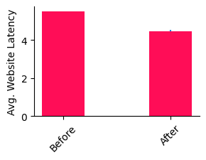
确实,我们获得了大约 1 秒的改善。我们还没有恢复正常运行,但我们已经缓解了部分问题。从这里开始,也许我们可以等到适当的修复程序部署。
附录:数据生成过程#
上述场景基于合成数据。正常数据是使用以下函数生成的
[16]:
from scipy.stats import truncexpon, halfnorm


def create_observed_latency_data(unobserved_intrinsic_latencies):
    observed_latencies = {}
    observed_latencies['Product DB'] = unobserved_intrinsic_latencies['Product DB']
    observed_latencies['Customer DB'] = unobserved_intrinsic_latencies['Customer DB']
    observed_latencies['Order DB'] = unobserved_intrinsic_latencies['Order DB']
    observed_latencies['Shipping Cost Service'] = unobserved_intrinsic_latencies['Shipping Cost Service']
    observed_latencies['Caching Service'] = np.random.choice([0, 1], size=(len(observed_latencies['Product DB']),),
                                                             p=[.5, .5]) * \
                                            observed_latencies['Product DB'] \
                                            + unobserved_intrinsic_latencies['Caching Service']
    observed_latencies['Product Service'] = np.maximum(np.maximum(observed_latencies['Shipping Cost Service'],
                                                                  observed_latencies['Caching Service']),
                                                       observed_latencies['Customer DB']) \
                                            + unobserved_intrinsic_latencies['Product Service']
    observed_latencies['Auth Service'] = observed_latencies['Customer DB'] \
                                         + unobserved_intrinsic_latencies['Auth Service']
    observed_latencies['Order Service'] = observed_latencies['Order DB'] \
                                          + unobserved_intrinsic_latencies['Order Service']
    observed_latencies['API'] = observed_latencies['Product Service'] \
                                + observed_latencies['Customer DB'] \
                                + observed_latencies['Auth Service'] \
                                + observed_latencies['Order Service'] \
                                + unobserved_intrinsic_latencies['API']
    observed_latencies['www'] = observed_latencies['API'] \
                                + observed_latencies['Auth Service'] \
                                + unobserved_intrinsic_latencies['www']
    observed_latencies['Website'] = observed_latencies['www'] \
                                    + unobserved_intrinsic_latencies['Website']

    return pd.DataFrame(observed_latencies)


def unobserved_intrinsic_latencies_normal(num_samples):
    return {
        'Website': truncexpon.rvs(size=num_samples, b=3, scale=0.2),
        'www': truncexpon.rvs(size=num_samples, b=2, scale=0.2),
        'API': halfnorm.rvs(size=num_samples, loc=0.5, scale=0.2),
        'Auth Service': halfnorm.rvs(size=num_samples, loc=0.1, scale=0.2),
        'Product Service': halfnorm.rvs(size=num_samples, loc=0.1, scale=0.2),
        'Order Service': halfnorm.rvs(size=num_samples, loc=0.5, scale=0.2),
        'Shipping Cost Service': halfnorm.rvs(size=num_samples, loc=0.1, scale=0.2),
        'Caching Service': halfnorm.rvs(size=num_samples, loc=0.1, scale=0.1),
        'Order DB': truncexpon.rvs(size=num_samples, b=5, scale=0.2),
        'Customer DB': truncexpon.rvs(size=num_samples, b=6, scale=0.2),
        'Product DB': truncexpon.rvs(size=num_samples, b=10, scale=0.2)
    }


normal_data = create_observed_latency_data(unobserved_intrinsic_latencies_normal(10000))
这模拟了在服务同步且没有同时影响两个节点的隐藏因素的假设下的延迟关系。此外,我们假设缓存服务只需在 50% 的情况下调用产品数据库(即缓存未命中率为 50%)。另外,我们假设产品服务可以并行调用其下游服务 Shipping Cost Service、Caching Service 和 Customer DB,并在所有三个服务返回后合并线程。
我们使用截断指数分布和半正态分布,因为它们的形状与实际服务中观察到的分布相似。
异常数据通过以下方式生成
[17]:
def unobserved_intrinsic_latencies_anomalous(num_samples):
    return {
        'Website': truncexpon.rvs(size=num_samples, b=3, scale=0.2),
        'www': truncexpon.rvs(size=num_samples, b=2, scale=0.2),
        'API': halfnorm.rvs(size=num_samples, loc=0.5, scale=0.2),
        'Auth Service': halfnorm.rvs(size=num_samples, loc=0.1, scale=0.2),
        'Product Service': halfnorm.rvs(size=num_samples, loc=0.1, scale=0.2),
        'Order Service': halfnorm.rvs(size=num_samples, loc=0.5, scale=0.2),
        'Shipping Cost Service': halfnorm.rvs(size=num_samples, loc=0.1, scale=0.2),
        'Caching Service': 2 + halfnorm.rvs(size=num_samples, loc=0.1, scale=0.1),
        'Order DB': truncexpon.rvs(size=num_samples, b=5, scale=0.2),
        'Customer DB': truncexpon.rvs(size=num_samples, b=6, scale=0.2),
        'Product DB': truncexpon.rvs(size=num_samples, b=10, scale=0.2)
    }

outlier_data = create_observed_latency_data(unobserved_intrinsic_latencies_anomalous(1000))
在这里,我们显着增加了Caching Service 的平均时间两秒,这与我们从 RCA 中得到的结果一致。请注意,Caching Service 中的高延迟会导致上游服务持续存在更高的延迟。特别是,客户会体验到比平时更高的延迟。