使用用户定义结果函数创建自定义反驳的简单示例

在此实验中，我们定义了一个线性数据集。为了找到系数，我们使用了线性回归估计器。为了测试线性估计器的有效性，我们现在将结果值替换为一个基于混杂因素值线性表达式产生的虚拟值。这有效地意味着处理对结果的影响应该为零。这正是我们应该从反驳器结果中期望的。

插入依赖项

from dowhy import CausalModel
import dowhy.datasets
import pandas as pd
import numpy as np

# Config dict to set the logging level
import logging.config
DEFAULT_LOGGING = {
    'version': 1,
    'disable_existing_loggers': False,
    'loggers': {
        '': {
            'level': 'WARN',
        },
    }
}

logging.config.dictConfig(DEFAULT_LOGGING)

创建数据集

您可以更改超参数的值，以查看随着每个参数的变化，效应如何改变 变量指南

变量名	数据类型	解释
\(Z_i\)	float	工具变量
\(W_i\)	float	混杂因素
\(v_0\)	float	处理
\(y\)	float	结果

# Value of the coefficient [BETA]
BETA = 10
# Number of Common Causes
NUM_COMMON_CAUSES = 2
# Number of Instruments
NUM_INSTRUMENTS = 1
# Number of Samples
NUM_SAMPLES = 100000
# Treatment is Binary
TREATMENT_IS_BINARY = False
data = dowhy.datasets.linear_dataset(beta=BETA,
                                 num_common_causes=NUM_COMMON_CAUSES,
                                 num_instruments=NUM_INSTRUMENTS,
                                 num_samples=NUM_SAMPLES,
                                 treatment_is_binary=TREATMENT_IS_BINARY)
data['df'].head()

	Z0	W0	W1	v0	y
0	1.0	0.483889	0.274341	12.245743	124.679058
1	0.0	1.774303	-0.569317	4.766134	50.185601
2	0.0	1.190897	0.429507	7.491711	79.542852
3	0.0	0.161984	-0.340266	-0.386472	-4.684053
4	0.0	-0.351776	-1.130420	-6.398013	-68.999834

创建因果模型

model = CausalModel(
    data = data['df'],
    treatment = data['treatment_name'],
    outcome = data['outcome_name'],
    graph = data['gml_graph'],
    instruments = data['instrument_names']
)

model.view_model()

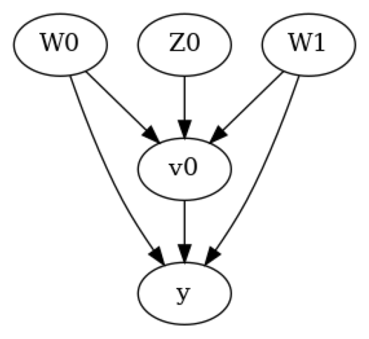
上图中，我们有一个因果图，显示了处理、结果、混杂因素和工具变量之间的关系。 - 混杂因素 \(W_0\) 和 \(W_1\) 影响处理和结果 - 工具变量 \(Z_0\) 通过处理 \(x\) 能够影响结果 \(y\)

识别估计量

identified_estimand = model.identify_effect(proceed_when_unidentifiable=True)
print(identified_estimand)

Estimand type: EstimandType.NONPARAMETRIC_ATE

### Estimand : 1
Estimand name: backdoor
Estimand expression:
  d
─────(E[y|W0,W1])
d[v₀]
Estimand assumption 1, Unconfoundedness: If U→{v0} and U→y then P(y|v0,W0,W1,U) = P(y|v0,W0,W1)

### Estimand : 2
Estimand name: iv
Estimand expression:
 ⎡                      -1⎤
 ⎢  d      ⎛  d        ⎞  ⎥
E⎢─────(y)⋅⎜─────([v₀])⎟  ⎥
 ⎣d[Z₀]    ⎝d[Z₀]      ⎠  ⎦
Estimand assumption 1, As-if-random: If U→→y then ¬(U →→{Z0})
Estimand assumption 2, Exclusion: If we remove {Z0}→{v0}, then ¬({Z0}→y)

### Estimand : 3
Estimand name: frontdoor
No such variable(s) found!

估计效应

causal_estimate = model.estimate_effect( identified_estimand,
                                       method_name="iv.instrumental_variable",
                                       method_params={'iv_instrument_name':'Z0'}
                                       )
print(causal_estimate)

*** Causal Estimate ***

## Identified estimand
Estimand type: EstimandType.NONPARAMETRIC_ATE

### Estimand : 1
Estimand name: iv
Estimand expression:
 ⎡                      -1⎤
 ⎢  d      ⎛  d        ⎞  ⎥
E⎢─────(y)⋅⎜─────([v₀])⎟  ⎥
 ⎣d[Z₀]    ⎝d[Z₀]      ⎠  ⎦
Estimand assumption 1, As-if-random: If U→→y then ¬(U →→{Z0})
Estimand assumption 2, Exclusion: If we remove {Z0}→{v0}, then ¬({Z0}→y)

## Realized estimand
Realized estimand: Wald Estimator
Realized estimand type: EstimandType.NONPARAMETRIC_ATE
Estimand expression:
 ⎡ d    ⎤
E⎢───(y)⎥
 ⎣dZ₀   ⎦
──────────
 ⎡ d     ⎤
E⎢───(v₀)⎥
 ⎣dZ₀    ⎦
Estimand assumption 1, As-if-random: If U→→y then ¬(U →→{Z0})
Estimand assumption 2, Exclusion: If we remove {Z0}→{v0}, then ¬({Z0}→y)
Estimand assumption 3, treatment_effect_homogeneity: Each unit's treatment ['v0'] is affected in the same way by common causes of ['v0'] and ['y']
Estimand assumption 4, outcome_effect_homogeneity: Each unit's outcome ['y'] is affected in the same way by common causes of ['v0'] and ['y']

Target units: ate

## Estimate
Mean value: 9.999108398071

反驳估计结果

使用随机生成的结果

ref = model.refute_estimate(identified_estimand,
                           causal_estimate,
                           method_name="dummy_outcome_refuter"
                           )
print(ref[0])

Refute: Use a Dummy Outcome
Estimated effect:0
New effect:-8.03184869278207e-05
p value:0.94

结果表明处理不会导致结果。估计的效应是一个趋近于零的值，这符合我们的预期。这表明，如果我们用随机生成的数据替换结果，估计器会正确预测处理的影响为零。

使用从混杂因素生成结果的函数

让我们定义一个简单的函数，将结果生成为混杂因素的线性函数。

coefficients = np.array([1,2])
bias = 3
def linear_gen(df):
    y_new = np.dot(df[['W0','W1']].values,coefficients) + 3
    return y_new

基本表达式的形式为 \(y_{new} = \beta_0W_0 + \beta_1W_1 + \gamma_0\)

其中，\(\beta_0=1\)，\(\beta_1=2\) 和 \(\gamma_0=3\)

ref = model.refute_estimate(identified_estimand,
                           causal_estimate,
                           method_name="dummy_outcome_refuter",
                           outcome_function=linear_gen
                           )

print(ref[0])

Refute: Use a Dummy Outcome
Estimated effect:0
New effect:9.03722497060772e-05
p value:0.8600000000000001

与之前的实验类似，我们观察到估计器显示处理的效应为零。反驳器证实了这一点，因为通过反驳获得的值非常低，并且在 100 次模拟中的 p 值 > 0.05。