401(k) 资格对净金融资产的影响#
在此案例研究中,我们将使用来自 401(k) 分析的真实世界数据,解释如何使用图因果模型估计平均处理效应 (ATE) 和条件平均处理效应 (CATE)。
背景#
20世纪80年代初,美国政府为雇员引入了几种税收递延储蓄方案,以鼓励个人为退休进行储蓄。其中一种流行的方案是 401(k) 计划,该计划允许雇员将一部分工资存入个人账户。本研究的目标是理解 401(k) 资格对净金融资产(即 401(k) 余额与非 401(k) 资产的总和)的影响,同时考虑个体特征(特别是收入)造成的异质性。
由于 401(k) 计划由雇主提供,只有提供此类计划的公司的雇员才有资格参与。因此,我们正在处理的是一项非随机化研究。有几个因素(例如教育程度、储蓄偏好)会影响 401(k) 资格以及净金融资产。
数据#
我们考虑了 1991 年收入和计划参与调查 (Survey of Income and Program Participation) 的一个样本。该样本包括参考个体年龄在 25-64 岁之间,且至少有一名个体受雇但无人个体经营的家庭。样本中有 9915 个家庭记录。每个家庭记录了 44 个变量,其中包括户主是否符合 401(k) 计划资格(处理)、净金融资产(结果),以及其他协变量,如年龄、收入、家庭规模、教育程度、婚姻状况等。我们特别考虑了其中的 16 个协变量。
下表总结了本案例研究中使用的变量。
变量名称 |
类型 |
详情 |
|---|---|---|
e401 |
处理 |
401(k) 计划资格 |
net_tfa |
结果 |
净金融资产(美元) |
age |
协变量 |
年龄 |
inc |
协变量 |
收入(美元) |
fsize |
协变量 |
家庭规模 |
educ |
协变量 |
教育年限 |
male |
协变量 |
是否男性? |
db |
协变量 |
固定收益养老金 |
marr |
协变量 |
是否已婚? |
twoearn |
协变量 |
双职工家庭 |
pira |
协变量 |
参与 IRA |
hown |
协变量 |
是否房主? |
hval |
协变量 |
房屋价值(美元) |
hequity |
协变量 |
房屋净值(美元) |
hmort |
协变量 |
房屋抵押贷款(美元) |
nohs |
协变量 |
未上高中?(独热编码) |
hs |
协变量 |
高中毕业?(独热编码) |
smcol |
协变量 |
上过大学?(独热编码) |
该数据集可从 `hdm <https://rdrr.io/cran/hdm/man/pension.html>`__ R 软件包在线公开获取。有关数据集的更多详细信息,请参阅以下论文
Chernohukov, C. Hansen (2004). 401(k) 参与对财富分布的影响:工具变量分位数回归分析。《经济与统计评论》86 (3), 735–751。
首先加载并分析数据。
[1]:
import pandas as pd
df = pd.read_csv("pension.csv")
[2]:
df.head()
[2]:
| ira | a401 | hval | hmort | hequity | nifa | net_nifa | tfa | net_tfa | tfa_he | ... | i3 | i4 | i5 | i6 | i7 | a1 | a2 | a3 | a4 | a5 | |
|---|---|---|---|---|---|---|---|---|---|---|---|---|---|---|---|---|---|---|---|---|---|
| 0 | 0 | 0 | 69000 | 60150 | 8850 | 100 | -3300 | 100 | -3300 | 5550 | ... | 1.0 | 0.0 | 0.0 | 0.0 | 0.0 | 0.0 | 1.0 | 0.0 | 0.0 | 0.0 |
| 1 | 0 | 0 | 78000 | 20000 | 58000 | 61010 | 61010 | 61010 | 61010 | 119010 | ... | 0.0 | 1.0 | 0.0 | 0.0 | 0.0 | 0.0 | 0.0 | 0.0 | 1.0 | 0.0 |
| 2 | 1800 | 0 | 200000 | 15900 | 184100 | 7549 | 7049 | 9349 | 8849 | 192949 | ... | 0.0 | 0.0 | 0.0 | 1.0 | 0.0 | 0.0 | 0.0 | 0.0 | 1.0 | 0.0 |
| 3 | 0 | 0 | 0 | 0 | 0 | 2487 | -6013 | 2487 | -6013 | -6013 | ... | 0.0 | 0.0 | 1.0 | 0.0 | 0.0 | 1.0 | 0.0 | 0.0 | 0.0 | 0.0 |
| 4 | 0 | 0 | 300000 | 90000 | 210000 | 10625 | -2375 | 10625 | -2375 | 207625 | ... | 0.0 | 1.0 | 0.0 | 0.0 | 0.0 | 0.0 | 0.0 | 1.0 | 0.0 | 0.0 |
5 行 × 44 列
401(k) 资格对净金融资产的影响(基于收入的条件分析)#
首先,我们构建一个因果图,包括 401(k) 计划资格(处理 \(T\))、净金融资产(结果 \(Y\))、我们假设能阻断 \(Y\) 和 \(T\) 之间所有后门路径的控制变量 \(W\),以及收入 \(X\)(我们希望基于此研究处理效应异质性的协变量)。
[3]:
import networkx as nx
import dowhy.gcm as gcm

treatment_var = "e401"
outcome_var = "net_tfa"
covariates = ["age","inc","fsize","educ","male","db",
              "marr","twoearn","pira","hown","hval",
              "hequity","hmort","nohs","hs","smcol"]

edges = [(treatment_var, outcome_var)]
edges.extend([(covariate, treatment_var) for covariate in covariates])
edges.extend([(covariate, outcome_var) for covariate in covariates])

# To ensure that the treatment is considered as a categorical variable, we convert the values explicitly to strings.
df = df.astype({treatment_var: str})

causal_graph = nx.DiGraph(edges)
[4]:
from dowhy.utils import plot

plot(causal_graph, figure_size=[20, 20])
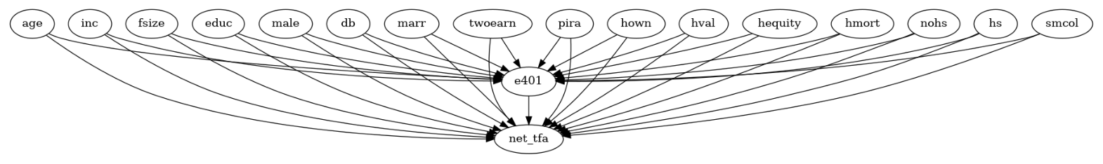
这里我们创建了一个简化图,其中协变量之间(即 \(X \cup W\) 中的节点)没有相互作用。在实践中,这很可能不是实际情况。然而,由于我们稍后直接从观测数据中获取协变量的联合样本来估计 CATE,我们可以忽略它们之间的相互作用。
在将因果模型分配给变量之前,我们先绘制它们的直方图,了解变量的分布情况。
[5]:
import matplotlib.pyplot as plt

cols = [treatment_var, outcome_var]
cols.extend(covariates)
plt.figure(figsize=(10,5))
for i, col in enumerate(cols):
    plt.subplot(3,6,i+1)
    plt.grid(False)
    plt.hist(df[col])
    plt.xlabel(col)
plt.tight_layout()
plt.show()
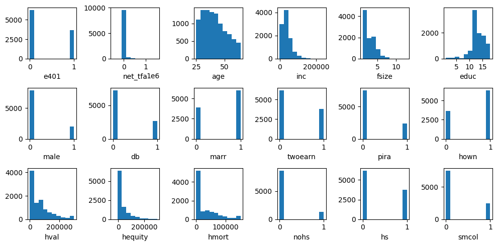
我们观察到实值变量不遵循诸如高斯分布等已知的参数分布。因此,对于没有父节点的变量,我们拟合经验分布,这对于分类变量也适用。
让我们明确地为每个节点分配因果机制。对于处理变量,我们使用随机森林分类器分配一个分类器函数式因果模型 (FCM)。对于结果变量,我们使用随机森林回归作为函数并为噪声分配经验分布,来分配一个加性噪声模型。由于因果图中其他变量没有父节点,我们为其分配经验分布。
[6]:
causal_model = gcm.StructuralCausalModel(causal_graph)
causal_model.set_causal_mechanism(treatment_var, gcm.ClassifierFCM(gcm.ml.create_random_forest_classifier()))
causal_model.set_causal_mechanism(outcome_var, gcm.AdditiveNoiseModel(gcm.ml.create_random_forest_regressor()))
for covariate in covariates:
    causal_model.set_causal_mechanism(covariate, gcm.EmpiricalDistribution())
如果我们没有先验知识或不熟悉统计学含义,也可以使用启发式方法自动分配因果机制
gcm.auto.assign_causal_mechanisms(causal_model, df)
这样,我们现在就可以从数据中拟合学习因果模型了。
[7]:
gcm.fit(causal_model, df)
Fitting causal mechanism of node smcol: 100%|██████████| 18/18 [00:06<00:00, 2.67it/s]
在计算 CATE 之前,我们首先将家庭按照收入百分位数划分为等宽的区间。这使得我们能够研究对不同收入群体的影响。
[8]:
import numpy as np

percentages = [0.0, 0.2, 0.4, 0.6, 0.8, 1.0]
bin_edges = [0]
bin_edges.extend(np.quantile(df.inc, percentages[1:]).tolist())
bin_edges[-1] += 1 # adding 1 to the last edge as last edge is excluded by np.digitize

groups = [f'{percentages[i]*100:.0f}%-{percentages[i+1]*100:.0f}%' for i in range(len(percentages)-1)]
group_index_to_group_label = dict(zip(range(1, len(bin_edges)+1), groups))
现在我们可以计算 CATE 了。为此,我们在已拟合的因果图中对处理变量进行随机干预,从干预分布中抽取样本,按收入组对观测结果进行分组,然后计算每组的处理效应。
[9]:
np.random.seed(47)

def estimate_cate():
    samples = gcm.interventional_samples(causal_model,
                                         {treatment_var: lambda x: np.random.choice(['0', '1'])},
                                         observed_data=df)
    eligible = samples[treatment_var] == '1'
    ate = samples[eligible][outcome_var].mean() - samples[~eligible][outcome_var].mean()
    result = dict(ate = ate)

    group_indices = np.digitize(samples['inc'], bin_edges)
    samples['group_index'] = group_indices

    for group_index in group_index_to_group_label:
        group_samples = samples[samples['group_index'] == group_index]
        eligible_in_group = group_samples[treatment_var] == '1'
        cate = group_samples[eligible_in_group][outcome_var].mean() - group_samples[~eligible_in_group][outcome_var].mean()
        result[group_index_to_group_label[group_index]] = cate

    return result

group_to_median, group_to_ci = gcm.confidence_intervals(estimate_cate, num_bootstrap_resamples=100)
print(group_to_median)
print(group_to_ci)
Estimating bootstrap interval...: 100%|██████████| 100/100 [00:43<00:00, 2.32it/s]
{'ate': 6524.583223183401, '0%-20%': 4010.8760624539045, '20%-40%': 3124.591365845997, '40%-60%': 5479.491988474934, '60%-80%': 7622.045252631407, '80%-100%': 12235.611495154653}
{'ate': array([4912.93938262, 8465.43365925]), '0%-20%': array([2612.44786522, 5582.21766875]), '20%-40%': array([1187.57446995, 5164.17566841]), '40%-60%': array([3333.67563274, 8129.58879172]), '60%-80%': array([ 4696.03425313, 10738.80810366]), '80%-100%': array([ 5083.79029031, 18774.95557817])}
401(k) 资格对净金融资产的平均处理效应是正向的,这由相应的置信区间表明。现在,让我们绘制不同收入组的 CATE 图,以便更清晰地了解情况。
[10]:
fig = plt.figure(figsize=(8,4))
for x, group in enumerate(groups):
    ci = group_to_ci[group]
    plt.plot((x, x), (ci[0], ci[1]), 'ro-', color='orange')
ax = fig.axes[0]
ax.spines['right'].set_visible(False)
ax.spines['top'].set_visible(False)
plt.xticks(range(len(groups)), groups)
plt.xlabel('Income group')
plt.ylabel('ATE of 401(k) eligibility on net financial assets')
plt.show()
/tmp/ipykernel_4333/1344202636.py:4: UserWarning: color is redundantly defined by the 'color' keyword argument and the fmt string "ro-" (-> color='r'). The keyword argument will take precedence.
  plt.plot((x, x), (ci[0], ci[1]), 'ro-', color='orange')
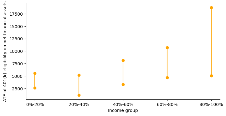
随着收入从低到高变化,影响也随之增加。这一结果似乎与不同收入群体的资源限制相符。