回归模型的敏感性分析#

敏感性分析帮助我们检查结果对未观测混杂可能性的敏感程度。实现了两种方法：1. Cinelli & Hazlett 的鲁棒性值 - 此方法仅支持线性回归估计器。 - 处理与结果的偏 R^2 显示了解释所有残余结果变异的混杂因素需要与处理有多强的关联才能消除估计效应。 - 鲁棒性值衡量未观测混杂因素需要与处理和结果具有的最小关联强度，以便改变结论。 - 鲁棒性值接近 1 意味着处理效应可以应对解释几乎所有处理和结果残余变异的强混杂因素。 - 鲁棒性值接近 0 意味着即使非常弱的混杂因素也可能改变结果。 - 基准测试检查因果推断对遗漏混杂因素合理强度的敏感性。 - 此方法基于 https://carloscinelli.com/files/Cinelli%20and%20Hazlett%20(2020)%20-%20Making%20Sense%20of%20Sensitivity.pdf 2. Ding & VanderWeele 的 E-值 - 此方法支持线性和逻辑回归。 - E-值是未测量混杂因素在风险比尺度上需要与处理和结果（在测量协变量的条件下）具有的最小关联强度，才能完全解释特定的处理-结果关联。 - 最小 E-值为 1，这意味着解释观测关联（即置信区间跨越零点）不需要未测量的混杂因素。 - 较高的 E-值意味着需要更强的未测量混杂因素来解释观测关联。没有最大的 E-值。 - McGowan & Greevy Jr 的根据测量协变量对 E-值进行基准测试。

步骤 1：加载所需软件包#

[1]:

import os, sys
sys.path.append(os.path.abspath("../../../"))
import dowhy
from dowhy import CausalModel
import pandas as pd
import numpy as np
import dowhy.datasets

# Config dict to set the logging level
import logging.config
DEFAULT_LOGGING = {
    'version': 1,
    'disable_existing_loggers': False,
    'loggers': {
        '': {
            'level': 'ERROR',
        },
    }
}

logging.config.dictConfig(DEFAULT_LOGGING)
# Disabling warnings output
import warnings
from sklearn.exceptions import DataConversionWarning
#warnings.filterwarnings(action='ignore', category=DataConversionWarning)

步骤 2：加载数据集#

我们创建一个数据集，其中共同原因与处理之间、以及共同原因与结果之间存在线性关系。Beta 是真实的因果效应。

[2]:

np.random.seed(100)
data = dowhy.datasets.linear_dataset( beta = 10,
                                      num_common_causes = 7,
                                      num_samples = 500,
                                      num_treatments = 1,
                                     stddev_treatment_noise =10,
                                     stddev_outcome_noise = 5
                                    )

[3]:

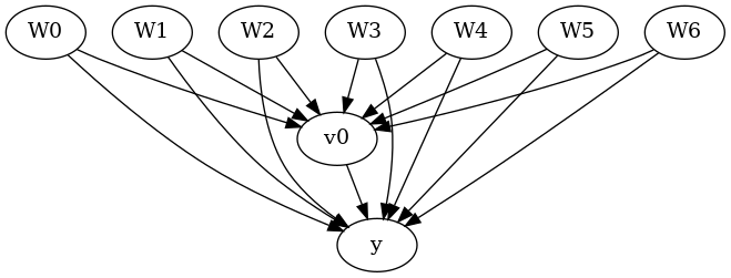
model = CausalModel(
            data=data["df"],
            treatment=data["treatment_name"],
            outcome=data["outcome_name"],
            graph=data["gml_graph"],
            test_significance=None,
        )
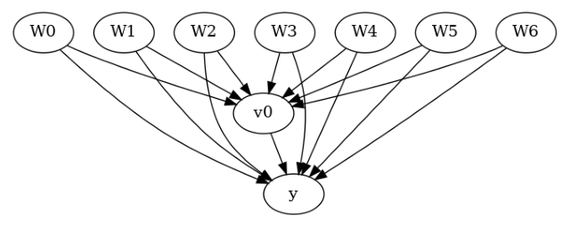
model.view_model()
from IPython.display import Image, display
display(Image(filename="causal_model.png"))
data['df'].head()

../_images/example_notebooks_sensitivity_analysis_testing_5_0.png

../_images/example_notebooks_sensitivity_analysis_testing_5_1.png

[3]:

	W0	W1	W2	W3	W4	W5	W6	v0	y
0	-0.145062	-0.235286	0.784843	0.869131	-1.567724	-1.290234	0.116096	True	1.386517
1	-0.228109	-0.020264	-0.589792	0.188139	-2.649265	-1.764439	-0.167236	False	-16.159402
2	0.868298	-1.097642	-0.109792	0.487635	-1.861375	-0.527930	-0.066542	False	-0.702560
3	-0.017115	1.123918	0.346060	1.845425	0.848049	0.778865	0.596496	True	27.714465
4	-0.757347	-1.426205	-0.457063	1.528053	-2.681410	0.394312	-0.687839	False	-20.082633

步骤 3：创建因果模型#

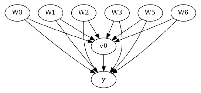
移除一个共同原因以模拟未观测混杂

[4]:

data["df"] = data["df"].drop("W4", axis = 1)
graph_str = 'graph[directed 1node[ id "y" label "y"]node[ id "W0" label "W0"] node[ id "W1" label "W1"] node[ id "W2" label "W2"] node[ id "W3" label "W3"]  node[ id "W5" label "W5"] node[ id "W6" label "W6"]node[ id "v0" label "v0"]edge[source "v0" target "y"]edge[ source "W0" target "v0"] edge[ source "W1" target "v0"] edge[ source "W2" target "v0"] edge[ source "W3" target "v0"] edge[ source "W5" target "v0"] edge[ source "W6" target "v0"]edge[ source "W0" target "y"] edge[ source "W1" target "y"] edge[ source "W2" target "y"] edge[ source "W3" target "y"] edge[ source "W5" target "y"] edge[ source "W6" target "y"]]'
model = CausalModel(
            data=data["df"],
            treatment=data["treatment_name"],
            outcome=data["outcome_name"],
            graph=graph_str,
            test_significance=None,
        )
model.view_model()
from IPython.display import Image, display
display(Image(filename="causal_model.png"))
data['df'].head()

../_images/example_notebooks_sensitivity_analysis_testing_7_0.png

../_images/example_notebooks_sensitivity_analysis_testing_7_1.png

[4]:

	W0	W1	W2	W3	W5	W6	v0	y
0	-0.145062	-0.235286	0.784843	0.869131	-1.290234	0.116096	True	1.386517
1	-0.228109	-0.020264	-0.589792	0.188139	-1.764439	-0.167236	False	-16.159402
2	0.868298	-1.097642	-0.109792	0.487635	-0.527930	-0.066542	False	-0.702560
3	-0.017115	1.123918	0.346060	1.845425	0.778865	0.596496	True	27.714465
4	-0.757347	-1.426205	-0.457063	1.528053	0.394312	-0.687839	False	-20.082633

步骤 4：识别#

[5]:

identified_estimand = model.identify_effect(proceed_when_unidentifiable=True)
print(identified_estimand)

Estimand type: EstimandType.NONPARAMETRIC_ATE

### Estimand : 1
Estimand name: backdoor
Estimand expression:
  d
─────(E[y|W3,W6,W1,W5,W0,W2])
d[v₀]
Estimand assumption 1, Unconfoundedness: If U→{v0} and U→y then P(y|v0,W3,W6,W1,W5,W0,W2,U) = P(y|v0,W3,W6,W1,W5,W0,W2)

### Estimand : 2
Estimand name: iv
No such variable(s) found!

### Estimand : 3
Estimand name: frontdoor
No such variable(s) found!

步骤 5：估计#

目前，线性敏感性分析仅支持线性回归估计器

[6]:

estimate = model.estimate_effect(identified_estimand,method_name="backdoor.linear_regression")
print(estimate)

*** Causal Estimate ***

## Identified estimand
Estimand type: EstimandType.NONPARAMETRIC_ATE

### Estimand : 1
Estimand name: backdoor
Estimand expression:
  d
─────(E[y|W3,W6,W1,W5,W0,W2])
d[v₀]
Estimand assumption 1, Unconfoundedness: If U→{v0} and U→y then P(y|v0,W3,W6,W1,W5,W0,W2,U) = P(y|v0,W3,W6,W1,W5,W0,W2)

## Realized estimand
b: y~v0+W3+W6+W1+W5+W0+W2
Target units: ate

## Estimate
Mean value: 10.697677486880925

步骤 6a：反驳和敏感性分析 - 方法 1#

identified_estimand: identifiedEstimand 类的一个实例，提供关于在处理影响结果时使用哪些因果路径的信息。 estimate: CausalEstimate 类的一个实例。从原始数据的估计器获得的估计值。 method_name: 反驳方法名称。 simulation_method: 线性敏感性分析使用“linear-partial-R2”。 benchmark_common_causes: 用于限制未观测混杂因素强度的协变量名称。 percent_change_estimate: 可能改变结果的处理估计值减少的百分比（默认值 = 1）。如果 percent_change_estimate = 1，则鲁棒性值描述了混杂因素与处理和结果关联的强度，以便将估计值减少 100%，即降至 0。 confounder_increases_estimate: confounder_increases_estimate = True 意味着混杂因素增加了估计值的绝对值，反之亦然。默认值为 confounder_increases_estimate = False，即考虑的混杂因素将估计值拉向零效应。 effect_fraction_on_treatment: 未观测混杂因素与处理之间的关联强度与基准协变量相比。 effect_fraction_on_outcome: 未观测混杂因素与结果之间的关联强度与基准协变量相比。 null_hypothesis_effect: 零假设下的假定效应（默认值 = 0）。 plot_estimate: 在执行敏感性分析时生成估计值的等高线图（默认值 = True）。要覆盖此设置，请将 plot_estimate 设置为 False。

[7]:

refute = model.refute_estimate(identified_estimand, estimate ,
                               method_name = "add_unobserved_common_cause",
                               simulation_method = "linear-partial-R2",
                               benchmark_common_causes = ["W3"],
                               effect_fraction_on_treatment = [ 1,2,3]
                              )

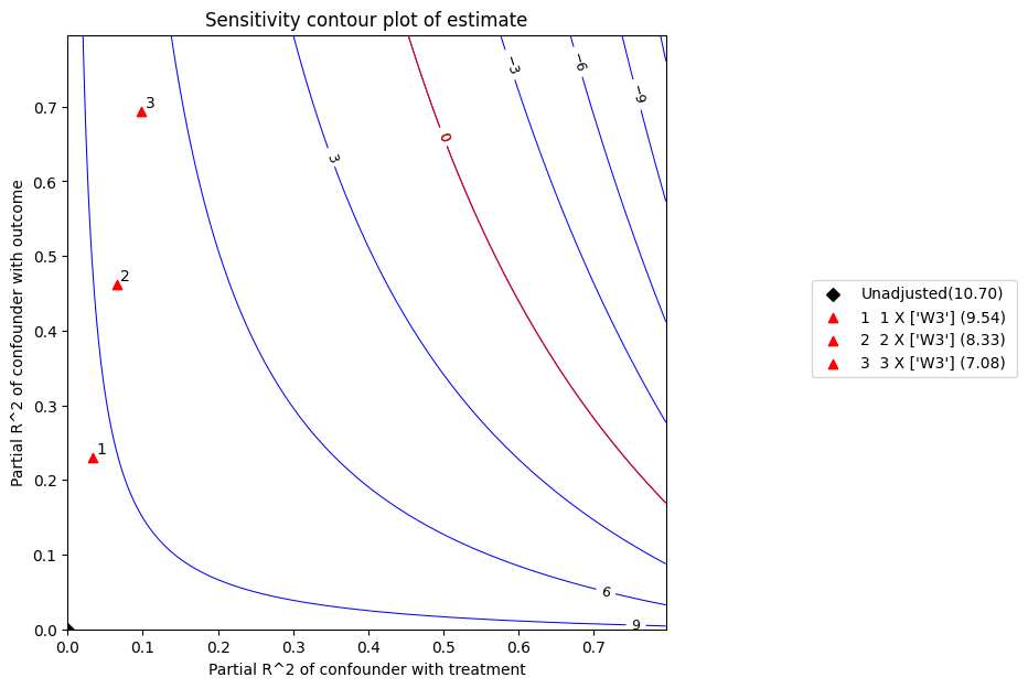
../_images/example_notebooks_sensitivity_analysis_testing_13_0.png

x 轴显示未观测混杂因素与处理的假设偏 R^2 值。y 轴显示未观测混杂因素与结果的假设偏 R^2 值。等高线水平代表将这些未观测混杂因素纳入完整回归模型时，其假设偏 R^2 值对应的调整 t-值或估计值。红线是临界阈值：具有此强度或更强的混杂因素足以使研究结论失效。

[8]:

refute.stats

[8]:

{'estimate': 10.697677486880925,
 'standard_error': 0.5938735661282949,
 'degree of freedom': 492,
 't_statistic': 18.013392238727626,
 'r2yt_w': 0.3974149837266683,
 'partial_f2': 0.6595168698094567,
 'robustness_value': 0.5467445572181009,
 'robustness_value_alpha': 0.5076289101030926}

[9]:

refute.benchmarking_results

[9]:

	r2tu_w	r2yu_tw	偏倚调整估计值	偏倚调整标准误	偏倚调整 t 值	偏倚调整置信区间下限	偏倚调整置信区间上限
0	0.032677	0.230238	9.535964	0.530308	17.981928	8.494016	10.577912
1	0.065354	0.461490	8.331381	0.451241	18.463243	7.444783	9.217979
2	0.098031	0.693855	7.080284	0.346341	20.443123	6.399795	7.760773

plot 函数参数列表#

plot_type: “estimate” 或 “t-value”。 critical_value: 将在图中突出显示的估计值或 t-值的特殊参考值。 x_limit: 图的 x 轴最大值（默认值 = 0.8）。 y_limit: 图的 y 轴最小值（默认值 = 0.8）。 num_points_per_contour: 计算和绘制每条等高线的点数（默认值 = 200）。 plot_size: 表示图大小的元组（默认值 = (7,7)）。 contours_color: 等高线颜色（默认值 = 蓝色）。字符串或数组。如果是数组，线条将按升序绘制特定颜色。 critical_contour_color: 阈值线颜色（默认值 = 红色）。 label_fontsize: 等高线标签字体大小（默认值 = 9）。 contour_linewidths: 等高线线宽（默认值 = 0.75）。 contour_linestyles: 等高线线型（默认值 = “solid”）。参见：https://matplotlib.net.cn/3.5.0/gallery/lines_bars_and_markers/linestyles.html。 contours_label_color: 等高线标签颜色（默认值 = 黑色）。 critical_label_color: 阈值线标签颜色（默认值 = 红色）。 unadjusted_estimate_marker: 图中未调整估计值的标记类型（默认值 = ‘D’）。参见：https://matplotlib.net.cn/stable/api/markers_api.html。 unadjusted_estimate_color: 图中未调整估计值的标记颜色（默认值 = “black”）。 adjusted_estimate_marker: 图中偏倚调整估计值的标记类型（默认值 = ‘^’）。adjusted_estimate_color: 图中偏倚调整估计值的标记颜色（默认值 = “red”）。 legend_position: 表示图例位置的元组（默认值 = (1.6, 0.6)）。

[10]:

refute.plot(plot_type = 't-value')

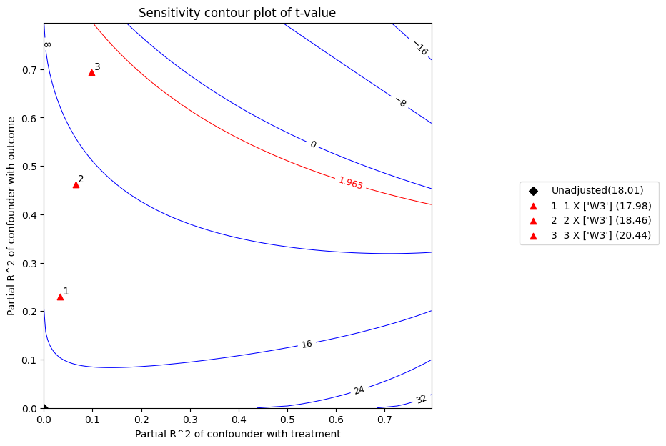
../_images/example_notebooks_sensitivity_analysis_testing_18_0.png

t 统计量是系数除以其标准误。t 值越高，拒绝零假设的证据越强。根据上面的图，在 5% 的显著性水平下，考虑到上述混杂因素，零效应的零假设将被拒绝。

[11]:

print(refute)

Sensitivity Analysis to Unobserved Confounding using R^2 paramterization

Unadjusted Estimates of Treatment ['v0'] :
Coefficient Estimate : 10.697677486880925
Degree of Freedom : 492
Standard Error : 0.5938735661282949
t-value : 18.013392238727626
F^2 value : 0.6595168698094567

Sensitivity Statistics :
Partial R2 of treatment with outcome : 0.3974149837266683
Robustness Value : 0.5467445572181009

Interpretation of results :
Any confounder explaining less than 54.67% percent of the residual variance of both the treatment and the outcome would not be strong enough to explain away the observed effect i.e bring down the estimate to 0

For a significance level of 5.0%, any confounder explaining more than 50.76% percent of the residual variance of both the treatment and the outcome would be strong enough to make the estimated effect not 'statistically significant'

If confounders explained 100% of the residual variance of the outcome, they would need to explain at least 39.74% of the residual variance of the treatment to bring down the estimated effect to 0

步骤 6b：反驳和敏感性分析 - 方法 2#

simulated_method_name: E-值为“e-value”

num_points_per_contour: 计算和绘制每条等高线的点数（默认值 = 200）
plot_size: 图的大小（默认值 = (6.4,4.8)）
contour_colors: 点估计和置信区间等高线的颜色（默认值 = [“blue”, “red”]）
xy_limit: 图的最大 x 和 y 值。默认值为 2 x E-值（默认值 = None）。

[12]:

refute = model.refute_estimate(identified_estimand, estimate ,
                               method_name = "add_unobserved_common_cause",
                               simulation_method = "e-value",
                              )

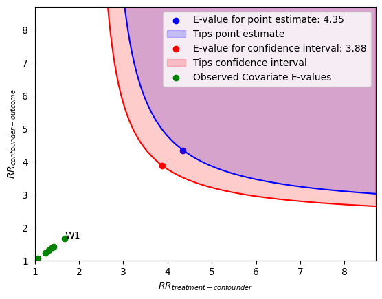
../_images/example_notebooks_sensitivity_analysis_testing_22_0.png

x 轴显示未测量混杂因素在不同处理水平下的风险比假设值。y 轴显示结果在不同混杂因素水平下的风险比假设值。
位于蓝色等高线之上或之上的点代表这些风险比的组合，这些组合将使点估计值发生变化（即解释掉）。
位于红色等高线之上或之上的点代表这些风险比的组合，这些组合将使置信区间发生变化（即解释掉）。
绿色点是观测协变量 E-值。它们衡量在剔除特定协变量并重新拟合估计器后，置信区间的界限在 E-值尺度上变化的程度。对应于最大观测协变量 E-值的协变量被标记出来。

[13]:

refute.stats

[13]:

{'converted_estimate': 2.4574470657354244,
 'converted_lower_ci': 2.2288567270043154,
 'converted_upper_ci': 2.7094815057979966,
 'evalue_estimate': 4.349958364289867,
 'evalue_lower_ci': 3.883832733630416,
 'evalue_upper_ci': None}

[14]:

refute.benchmarking_results

[14]:

	converted_est	converted_lower_ci	converted_upper_ci	observed_covariate_e_value
dropped_covariate
W1	2.992523	2.666604	3.358276	1.681140
W6	2.687656	2.446341	2.952774	1.424835
W3	2.692807	2.422402	2.993396	1.394043
W0	2.599868	2.368550	2.853776	1.320751
W5	2.553701	2.315245	2.816716	1.239411
W2	2.473648	2.217699	2.759138	1.076142

[15]:

print(refute)

Sensitivity Analysis to Unobserved Confounding using the E-value

Unadjusted Estimates of Treatment: v0
Estimate (converted to risk ratio scale): 2.4574470657354244
Lower 95% CI (converted to risk ratio scale): 2.2288567270043154
Upper 95% CI (converted to risk ratio scale): 2.7094815057979966

Sensitivity Statistics:
E-value for point estimate: 4.349958364289867
E-value for lower 95% CI: 3.883832733630416
E-value for upper 95% CI: None
Largest Observed Covariate E-value: 1.6811401167656765 (W1)

Interpretation of results:
Unmeasured confounder(s) would have to be associated with a 4.35-fold increase in the risk of y, and must be 4.35 times more prevalent in v0, to explain away the observed point estimate.
Unmeasured confounder(s) would have to be associated with a 3.88-fold increase in the risk of y, and must be 3.88 times more prevalent in v0, to explain away the observed confidence interval.

现在，我们在相同的数据集上运行敏感性分析，但不剔除任何变量。我们得到的鲁棒性值从 0.55 变为 0.95，这意味着处理效应可以应对解释处理和结果几乎所有残余变异的强混杂因素。

[16]:

np.random.seed(100)
data = dowhy.datasets.linear_dataset( beta = 10,
                                      num_common_causes = 7,
                                      num_samples = 500,
                                      num_treatments = 1,
                                     stddev_treatment_noise=10,
                                     stddev_outcome_noise = 1
                                    )

[17]:

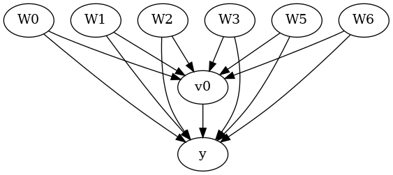
model = CausalModel(
            data=data["df"],
            treatment=data["treatment_name"],
            outcome=data["outcome_name"],
            graph=data["gml_graph"],
            test_significance=None,
        )
model.view_model()
from IPython.display import Image, display
display(Image(filename="causal_model.png"))
data['df'].head()

../_images/example_notebooks_sensitivity_analysis_testing_29_0.png

../_images/example_notebooks_sensitivity_analysis_testing_29_1.png

[17]:

	W0	W1	W2	W3	W4	W5	W6	v0	y
0	-0.145062	-0.235286	0.784843	0.869131	-1.567724	-1.290234	0.116096	True	6.311809
1	-0.228109	-0.020264	-0.589792	0.188139	-2.649265	-1.764439	-0.167236	False	-12.274406
2	0.868298	-1.097642	-0.109792	0.487635	-1.861375	-0.527930	-0.066542	False	-6.487561
3	-0.017115	1.123918	0.346060	1.845425	0.848049	0.778865	0.596496	True	24.653183
4	-0.757347	-1.426205	-0.457063	1.528053	-2.681410	0.394312	-0.687839	False	-13.770396

[18]:

identified_estimand = model.identify_effect(proceed_when_unidentifiable=True)
print(identified_estimand)

Estimand type: EstimandType.NONPARAMETRIC_ATE

### Estimand : 1
Estimand name: backdoor
Estimand expression:
  d
─────(E[y|W3,W6,W1,W5,W0,W4,W2])
d[v₀]
Estimand assumption 1, Unconfoundedness: If U→{v0} and U→y then P(y|v0,W3,W6,W1,W5,W0,W4,W2,U) = P(y|v0,W3,W6,W1,W5,W0,W4,W2)

### Estimand : 2
Estimand name: iv
No such variable(s) found!

### Estimand : 3
Estimand name: frontdoor
No such variable(s) found!

[19]:

estimate = model.estimate_effect(identified_estimand,method_name="backdoor.linear_regression")
print(estimate)

*** Causal Estimate ***

## Identified estimand
Estimand type: EstimandType.NONPARAMETRIC_ATE

### Estimand : 1
Estimand name: backdoor
Estimand expression:
  d
─────(E[y|W3,W6,W1,W5,W0,W4,W2])
d[v₀]
Estimand assumption 1, Unconfoundedness: If U→{v0} and U→y then P(y|v0,W3,W6,W1,W5,W0,W4,W2,U) = P(y|v0,W3,W6,W1,W5,W0,W4,W2)

## Realized estimand
b: y~v0+W3+W6+W1+W5+W0+W4+W2
Target units: ate

## Estimate
Mean value: 10.081924375588297

[20]:

refute = model.refute_estimate(identified_estimand, estimate ,
                               method_name = "add_unobserved_common_cause",
                               simulation_method = "linear-partial-R2",
                               benchmark_common_causes = ["W3"],
                               effect_fraction_on_treatment = [ 1,2,3])

/__w/dowhy/dowhy/dowhy/causal_refuters/linear_sensitivity_analyzer.py:199: RuntimeWarning: divide by zero encountered in divide
  bias_adjusted_t = (bias_adjusted_estimate - self.null_hypothesis_effect) / bias_adjusted_se
/__w/dowhy/dowhy/dowhy/causal_refuters/linear_sensitivity_analyzer.py:201: RuntimeWarning: invalid value encountered in divide
  bias_adjusted_partial_r2 = bias_adjusted_t**2 / (

../_images/example_notebooks_sensitivity_analysis_testing_32_1.png

[21]:

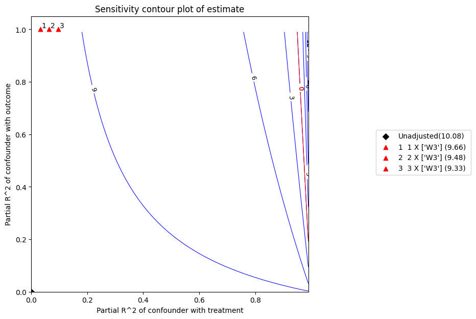
refute.plot(plot_type = 't-value')

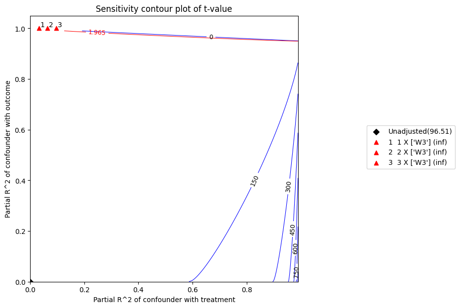
../_images/example_notebooks_sensitivity_analysis_testing_33_0.png

[22]:

print(refute)

Sensitivity Analysis to Unobserved Confounding using R^2 paramterization

Unadjusted Estimates of Treatment ['v0'] :
Coefficient Estimate : 10.081924375588297
Degree of Freedom : 491
Standard Error : 0.10446229543424744
t-value : 96.51256784735547
F^2 value : 18.970826379817503

Sensitivity Statistics :
Partial R2 of treatment with outcome : 0.9499269594066173
Robustness Value : 0.9522057801012398

Interpretation of results :
Any confounder explaining less than 95.22% percent of the residual variance of both the treatment and the outcome would not be strong enough to explain away the observed effect i.e bring down the estimate to 0

For a significance level of 5.0%, any confounder explaining more than 95.04% percent of the residual variance of both the treatment and the outcome would be strong enough to make the estimated effect not 'statistically significant'

If confounders explained 100% of the residual variance of the outcome, they would need to explain at least 94.99% of the residual variance of the treatment to bring down the estimated effect to 0

[23]:

refute.stats

[23]:

{'estimate': 10.081924375588297,
 'standard_error': 0.10446229543424744,
 'degree of freedom': 491,
 't_statistic': 96.51256784735547,
 'r2yt_w': 0.9499269594066173,
 'partial_f2': 18.970826379817503,
 'robustness_value': 0.9522057801012398,
 'robustness_value_alpha': 0.950386691319526}

[24]:

refute.benchmarking_results

[24]:

	r2tu_w	r2yu_tw	偏倚调整估计值	偏倚调整 t 值	偏倚调整置信区间下限	偏倚调整置信区间上限
0	0.031976	1.0	9.661229	inf	9.661229	9.661229
1	0.063952	1.0	9.476895	inf	9.476895	9.476895
2	0.095927	1.0	9.327927	inf	9.327927	9.327927