寻找最优调整集#
预备知识#
本笔记本演示了 Smucler, Sapienza 和 Rotnitzky (Biometrika, 2022) 以及 Smucler 和 Rotnitzky (Journal of Causal Inference, 2022) 中开发的算法的使用,用于计算在各种约束下能够产生干预均值及其对比(如 ATE)的有效估计量的后门集。我们首先回顾这些论文中的一些定义。我们省略了大部分技术细节,并请读者查阅原始论文以获取更多信息。
**最优后门集**是由可观测变量组成的后门集,在基于可观测后门集的非参数干预均值估计量中,它产生具有最小渐近方差的估计量。当没有潜变量时,这种最优后门集总是存在,并且算法在这种情况下保证能够计算出它。在具有潜变量的非参数图模型下,这种后门集可能不存在。
**最优最小后门集**是由可观测变量组成的最小后门集,在基于可观测最小后门集的非参数干预均值估计量中,它产生具有最小渐近方差的估计量。
**最优最小成本后门集**是由可观测变量组成的最小成本后门集,在基于可观测最小成本后门集的非参数干预均值估计量中,它产生具有最小渐近方差的估计量。后门集的成本定义为构成该集合的变量成本之和。请注意,当所有成本相等时,最优最小成本后门集等同于具有最小基数的最优后门集。
根据 Henckel, Perkovic 和 Maathuis (JRSS B, 2022) 的结果,这些不同的最优后门集不仅在非参数图模型和非参数干预均值估计量下是最优的,而且在线性图模型和 OLS 估计量下也是最优的。
观察性研究的设计#
[1]:
from dowhy.causal_graph import CausalGraph
from dowhy.causal_identifier import AutoIdentifier, BackdoorAdjustment, EstimandType
from dowhy.graph import build_graph_from_str
from dowhy.utils.plotting import plot
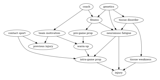
考虑 Shrier & Platt (2008) 中讨论的以下假设观察性研究的设计。该研究的目的是评估热身运动对运动后受伤的影响。假设研究人员推测下图代表了一个因果图模型。节点 warm-up 是处理变量,代表运动员在运动前进行的运动类型;节点 injury 代表结果变量。
假设研究的目标是估计和比较不同个体化治疗规则对应的干预均值。每条规则根据先前的伤病和团队动力来规定热身运动的类型。例如,一条这样的规则可能是当患者先前的伤病为 1 且团队动力 > 6 时,安排其进行柔和的热身运动,但任何其他(可能是随机的)先前的伤病和团队动力的函数来设置处理变量也可能是有意义的。更正式地说,研究的目标是,对于上述某些政策集合,在一个所有患者根据其中一条政策分配到一种治疗方式的世界中,估计结果的均值。此外,我们假设由于实际限制,无法测量基因、赛前本体感觉、赛中本体感觉和组织薄弱等变量。本体感觉是指个体感知自己身体的运动、动作和位置的能力。
要构建图,我们首先创建一个字符串来声明图的节点和边。然后,我们创建一个包含所有可观测变量的列表,在本例中,即图中除 genetics、pre-game proprioception、intra-game proprioception 和 tissue weakness 之外的所有变量。然后,我们将所有这些信息传递给 CausalGraph 类,以创建其一个实例。
[2]:
graph_str = """graph[directed 1 node[id "coach" label "coach"]
                        node[id "team motivation" label "team motivation"]
                        node[id "fitness" label "fitness"]
                        node[id "pre-game prop" label "pre-game prop"]
                        node[id "intra-game prop" label "intra-game prop"]
                        node[id "neuromusc fatigue" label "neuromusc fatigue"]
                        node[id "warm-up" label "warm-up"]
                        node[id "previous injury" label "previous injury"]
                        node[id "contact sport" label "contact sport"]
                        node[id "genetics" label "genetics"]
                        node[id "injury" label "injury"]
                        node[id "tissue disorder" label "tissue disorder"]
                        node[id "tissue weakness" label "tissue weakness"]
                        edge[source "coach" target "team motivation"]
                        edge[source "coach" target "fitness"]
                        edge[source "fitness" target "pre-game prop"]
                        edge[source "fitness" target "neuromusc fatigue"]
                        edge[source "team motivation" target "warm-up"]
                        edge[source "team motivation" target "previous injury"]
                        edge[source "pre-game prop" target "warm-up"]
                        edge[source "warm-up" target "intra-game prop"]
                        edge[source "contact sport" target "previous injury"]
                        edge[source "contact sport" target "intra-game prop"]
                        edge[source "intra-game prop" target "injury"]
                        edge[source "genetics" target "fitness"]
                        edge[source "genetics" target "neuromusc fatigue"]
                        edge[source "genetics" target "tissue disorder"]
                        edge[source "tissue disorder" target "neuromusc fatigue"]
                        edge[source "tissue disorder" target "tissue weakness"]
                        edge[source "neuromusc fatigue" target "intra-game prop"]
                        edge[source "neuromusc fatigue" target "injury"]
                        edge[source "tissue weakness" target "injury"]
                        ]
"""
observed_node_names = [
    "coach",
    "team motivation",
    "fitness",
    "neuromusc fatigue",
    "warm-up",
    "previous injury",
    "contact sport",
    "tissue disorder",
    "injury",
]
treatment_name = "warm-up"
outcome_name = "injury"
G = build_graph_from_str(graph_str)
我们可以使用 view_graph 方法轻松创建图的绘制。
[3]:
plot(G)
接下来,我们演示如何使用 CausalIdentifier 类计算上述示例图中预备知识部分定义的后门集。要计算最优后门集、最优最小后门集和最优最小成本后门集,我们需要实例化 CausalIdentifier 类的对象,将 method_name 参数分别设置为“efficient-adjustment”、“efficient-minimal-adjustment”和“efficient-mincost-adjustment”。然后,我们需要调用 identify_effect 方法,将条件节点列表作为参数传入,即用于决定如何分配处理的节点。如上所述,在本例中,这些节点是 previous injury 和 team motivation。对于我们不关心个体化干预的设置,我们可以只传入一个空列表作为条件节点。
[4]:
conditional_node_names = ["previous injury", "team motivation"]
[5]:
ident_eff = AutoIdentifier(
    estimand_type=EstimandType.NONPARAMETRIC_ATE,
    backdoor_adjustment=BackdoorAdjustment.BACKDOOR_EFFICIENT,
)
print(
    ident_eff.identify_effect(
        graph=G,
        action_nodes=treatment_name,
        outcome_nodes=outcome_name,
        observed_nodes=observed_node_names,
        conditional_node_names=conditional_node_names
    )
)
Estimand type: EstimandType.NONPARAMETRIC_ATE

### Estimand : 1
Estimand name: backdoor
Estimand expression:
    d                                                                          ↪
──────────(E[injury|previous injury,neuromusc fatigue,tissue disorder,contact  ↪
d[warm-up]                                                                     ↪

↪
↪ sport,team motivation])
↪
Estimand assumption 1, Unconfoundedness: If U→{warm-up} and U→injury then P(injury|warm-up,previous injury,neuromusc fatigue,tissue disorder,contact sport,team motivation,U) = P(injury|warm-up,previous injury,neuromusc fatigue,tissue disorder,contact sport,team motivation)

### Estimand : 2
Estimand name: iv
No such variable(s) found!

### Estimand : 3
Estimand name: frontdoor
No such variable(s) found!
因此,最优后门集由 previous injury、neuromusc fatigue、team motivation、tissue disorder 和 contact sport 组成。
类似地,我们可以计算最优最小后门集。
[6]:
ident_minimal_eff = AutoIdentifier(
    estimand_type=EstimandType.NONPARAMETRIC_ATE,
    backdoor_adjustment=BackdoorAdjustment.BACKDOOR_MIN_EFFICIENT,
)
print(
    ident_minimal_eff.identify_effect(
        graph=G,
        action_nodes=treatment_name,
        outcome_nodes=outcome_name,
        observed_nodes=observed_node_names,
        conditional_node_names=conditional_node_names
    )
)
Estimand type: EstimandType.NONPARAMETRIC_ATE

### Estimand : 1
Estimand name: backdoor
Estimand expression:
    d                                                                          ↪
──────────(E[injury|team motivation,neuromusc fatigue,tissue disorder,previous ↪
d[warm-up]                                                                     ↪

↪
↪  injury])
↪
Estimand assumption 1, Unconfoundedness: If U→{warm-up} and U→injury then P(injury|warm-up,team motivation,neuromusc fatigue,tissue disorder,previous injury,U) = P(injury|warm-up,team motivation,neuromusc fatigue,tissue disorder,previous injury)

### Estimand : 2
Estimand name: iv
No such variable(s) found!

### Estimand : 3
Estimand name: frontdoor
No such variable(s) found!
最后,我们可以计算最优最小成本后门集。由于此图的节点没有关联任何成本,我们将不会向 identify_effect 传入任何成本。该方法将发出警告,将成本设置为 1,并计算最优最小成本后门集,如上所述,在这种情况下,它与最小基数的最优后门集一致。
[7]:
ident_mincost_eff = AutoIdentifier(
    estimand_type=EstimandType.NONPARAMETRIC_ATE,
    backdoor_adjustment=BackdoorAdjustment.BACKDOOR_MINCOST_EFFICIENT,
)
print(
    ident_mincost_eff.identify_effect(
        graph=G,
        action_nodes=treatment_name,
        outcome_nodes=outcome_name,
        observed_nodes=observed_node_names,
        conditional_node_names=conditional_node_names
    )
)
Estimand type: EstimandType.NONPARAMETRIC_ATE

### Estimand : 1
Estimand name: backdoor
Estimand expression:
    d
──────────(E[injury|team motivation,fitness,previous injury])
d[warm-up]
Estimand assumption 1, Unconfoundedness: If U→{warm-up} and U→injury then P(injury|warm-up,team motivation,fitness,previous injury,U) = P(injury|warm-up,team motivation,fitness,previous injury)

### Estimand : 2
Estimand name: iv
No such variable(s) found!

### Estimand : 3
Estimand name: frontdoor
No such variable(s) found!
稍后,我们将为节点关联成本的图计算最优最小成本后门集。
无法保证存在最优后门集的充分条件的示例#
Smucler, Sapienza 和 Rotnitzky (Biometrika, 2022) 证明,当所有变量都是可观测的,或者当所有可观测变量是处理、结果或条件节点的祖先时,可以仅基于图找到最优后门集,并提供了一个计算算法。这正是上述示例中实现的算法。
然而,存在仅凭图准则无法找到可观测的最优后门集的情况。对于下图,Rotnitzky 和 Smucler (JMLR, 2021) 在他们的示例 5 中表明,取决于生成数据的规律,最优后门集可能由 Z1 和 Z2 组成,或者是一个空集。更精确地说,他们表明存在与图兼容的概率规律,在这种规律下 {Z1, Z2} 是最有效的调整集,而在其他概率规律下,空集是最有效的调整集;遗憾的是,仅凭图本身无法判断两者中哪个更好。
请注意,在此图中,上述关于最优后门集存在的充分条件不成立,因为 Z2 是可观测的,但不是处理结果或条件节点(本例中为空集)的祖先。
另一方面,Smucler, Sapienza 和 Rotnitzky (Biometrika, 2022) 表明,只要存在至少一个由可观测变量组成的后门集,最优最小和最优最小成本(基数)可观测后门集总是存在的。也就是说,当搜索仅限于最小或最小成本(基数)后门集时,上述情况不会发生,并且始终可以仅基于图准则检测到最有效的后门集。
对于此示例,调用 CausalIdentifier 实例的 identify_effect 方法,并将属性 method_name 设置为“efficient-adjustment”将引发错误。对于此图,最优最小后门集和最优最小基数后门集都等于空集。
[8]:
graph_str = """graph[directed 1 node[id "X" label "X"]
                        node[id "Y" label "Y"]
                        node[id "Z1" label "Z1"]
                        node[id "Z2" label "Z2"]
                        node[id "U" label "U"]
                        edge[source "X" target "Y"]
                        edge[source "Z1" target "X"]
                        edge[source "Z1" target "Z2"]
                        edge[source "U" target "Z2"]
                        edge[source "U" target "Y"]
                        ]
"""
observed_node_names = ["X", "Y", "Z1", "Z2"]
treatment_name = "X"
outcome_name = "Y"
G = build_graph_from_str(graph_str)
在此示例中,处理干预是静态的,因此没有条件节点。
[9]:
ident_eff = AutoIdentifier(
    estimand_type=EstimandType.NONPARAMETRIC_ATE,
    backdoor_adjustment=BackdoorAdjustment.BACKDOOR_EFFICIENT,
)
try:
    results_eff = ident_eff.identify_effect(graph=G,
                                            action_nodes=treatment_name,
                                            outcome_nodes=outcome_name,
                                            observed_nodes=observed_node_names)
except ValueError as e:
    print(e)
Conditions to guarantee the existence of an optimal adjustment set are not satisfied
[10]:
ident_eff = AutoIdentifier(
    estimand_type=EstimandType.NONPARAMETRIC_ATE,
    backdoor_adjustment=BackdoorAdjustment.BACKDOOR_MIN_EFFICIENT,
)
print(
    ident_minimal_eff.identify_effect(
        graph=G,
        action_nodes=treatment_name,
        outcome_nodes=outcome_name,
        observed_nodes=observed_node_names
    )
)
Estimand type: EstimandType.NONPARAMETRIC_ATE

### Estimand : 1
Estimand name: backdoor
Estimand expression:
 d
────(E[Y])
d[X]
Estimand assumption 1, Unconfoundedness: If U→{X} and U→Y then P(Y|X,,U) = P(Y|X,)

### Estimand : 2
Estimand name: iv
Estimand expression:
 ⎡                     -1⎤
 ⎢  d      ⎛  d       ⎞  ⎥
E⎢─────(Y)⋅⎜─────([X])⎟  ⎥
 ⎣d[Z₁]    ⎝d[Z₁]     ⎠  ⎦
Estimand assumption 1, As-if-random: If U→→Y then ¬(U →→{Z1})
Estimand assumption 2, Exclusion: If we remove {Z1}→{X}, then ¬({Z1}→Y)

### Estimand : 3
Estimand name: frontdoor
No such variable(s) found!
[11]:
ident_eff = AutoIdentifier(
    estimand_type=EstimandType.NONPARAMETRIC_ATE,
    backdoor_adjustment=BackdoorAdjustment.BACKDOOR_MINCOST_EFFICIENT,
)
print(
    ident_mincost_eff.identify_effect(
        graph=G,
        action_nodes=treatment_name,
        outcome_nodes=outcome_name,
        observed_nodes=observed_node_names
    )
)
Estimand type: EstimandType.NONPARAMETRIC_ATE

### Estimand : 1
Estimand name: backdoor
Estimand expression:
 d
────(E[Y])
d[X]
Estimand assumption 1, Unconfoundedness: If U→{X} and U→Y then P(Y|X,,U) = P(Y|X,)

### Estimand : 2
Estimand name: iv
Estimand expression:
 ⎡                     -1⎤
 ⎢  d      ⎛  d       ⎞  ⎥
E⎢─────(Y)⋅⎜─────([X])⎟  ⎥
 ⎣d[Z₁]    ⎝d[Z₁]     ⎠  ⎦
Estimand assumption 1, As-if-random: If U→→Y then ¬(U →→{Z1})
Estimand assumption 2, Exclusion: If we remove {Z1}→{X}, then ¬({Z1}→Y)

### Estimand : 3
Estimand name: frontdoor
No such variable(s) found!
不存在可观测调整集的示例#
在下图中,不存在仅由可观测变量组成的调整集。在这种设置下,使用上述任何方法都将引发错误。
[12]:
graph_str = """graph[directed 1 node[id "X" label "X"]
                        node[id "Y" label "Y"]
                        node[id "U" label "U"]
                        edge[source "X" target "Y"]
                        edge[source "U" target "X"]
                        edge[source "U" target "Y"]
                        ]
"""
observed_node_names = ["X", "Y"]
treatment_name = "X"
outcome_name = "Y"
G = build_graph_from_str(graph_str)
[13]:
ident_eff = AutoIdentifier(
    estimand_type=EstimandType.NONPARAMETRIC_ATE,
    backdoor_adjustment=BackdoorAdjustment.BACKDOOR_EFFICIENT,
)
try:
    results_eff = ident_eff.identify_effect(
        graph=G,
        action_nodes=treatment_name,
        outcome_nodes=outcome_name,
        observed_nodes=observed_node_names
    )
except ValueError as e:
    print(e)
An adjustment set formed by observable variables does not exist
带有成本的示例#
这是 Smucler 和 Rotnitzky (Journal of Causal Inference, 2022) 图 1 和图 2 中的图。这里我们假设可观测变量关联了正成本。
[14]:
graph_str = """graph[directed 1 node[id "L" label "L"]
                        node[id "X" label "X"]
                        node[id "K" label "K"]
                        node[id "B" label "B"]
                        node[id "Q" label "Q"]
                        node[id "R" label "R"]
                        node[id "T" label "T"]
                        node[id "M" label "M"]
                        node[id "Y" label "Y"]
                        node[id "U" label "U"]
                        node[id "F" label "F"]
                        edge[source "L" target "X"]
                        edge[source "X" target "M"]
                        edge[source "K" target "X"]
                        edge[source "B" target "K"]
                        edge[source "B" target "R"]
                        edge[source "Q" target "K"]
                        edge[source "Q" target "T"]
                        edge[source "R" target "Y"]
                        edge[source "T" target "Y"]
                        edge[source "M" target "Y"]
                        edge[source "U" target "Y"]
                        edge[source "U" target "F"]
                        ]
                        """
observed_node_names = ["L", "X", "B", "K", "Q", "R", "M", "T", "Y", "F"]
conditional_node_names = ["L"]
costs = [
    ("L", {"cost": 1}),
    ("B", {"cost": 1}),
    ("K", {"cost": 4}),
    ("Q", {"cost": 1}),
    ("R", {"cost": 2}),
    ("T", {"cost": 1}),
]
G = build_graph_from_str(graph_str)
请注意,在这种情况下,我们将 conditional_node_names 列表和 costs 列表都传递给了 identify_effect 方法。
[15]:
ident_eff = AutoIdentifier(
    estimand_type=EstimandType.NONPARAMETRIC_ATE,
    backdoor_adjustment=BackdoorAdjustment.BACKDOOR_MINCOST_EFFICIENT,
    costs=costs,
)
print(
    ident_mincost_eff.identify_effect(
        graph=G,
        action_nodes=treatment_name,
        outcome_nodes=outcome_name,
        observed_nodes=observed_node_names,
        conditional_node_names=conditional_node_names
    )
)
Estimand type: EstimandType.NONPARAMETRIC_ATE

### Estimand : 1
Estimand name: backdoor
Estimand expression:
 d
────(E[Y|K,L])
d[X]
Estimand assumption 1, Unconfoundedness: If U→{X} and U→Y then P(Y|X,K,L,U) = P(Y|X,K,L)

### Estimand : 2
Estimand name: iv
Estimand expression:
 ⎡                   -1⎤
 ⎢ d      ⎛ d       ⎞  ⎥
E⎢────(Y)⋅⎜────([X])⎟  ⎥
 ⎣d[L]    ⎝d[L]     ⎠  ⎦
Estimand assumption 1, As-if-random: If U→→Y then ¬(U →→{L})
Estimand assumption 2, Exclusion: If we remove {L}→{X}, then ¬({L}→Y)

### Estimand : 3
Estimand name: frontdoor
Estimand expression:
 ⎡ d       d       ⎤
E⎢────(Y)⋅────([M])⎥
 ⎣d[M]    d[X]     ⎦
Estimand assumption 1, Full-mediation: M intercepts (blocks) all directed paths from X to Y.
Estimand assumption 2, First-stage-unconfoundedness: If U→{X} and U→{M} then P(M|X,U) = P(M|X)
Estimand assumption 3, Second-stage-unconfoundedness: If U→{M} and U→Y then P(Y|M, X, U) = P(Y|M, X)
我们还计算了最优最小后门集,在这种情况下,它与最优最小成本后门集不同。
[16]:
ident_eff = AutoIdentifier(
    estimand_type=EstimandType.NONPARAMETRIC_ATE,
    backdoor_adjustment=BackdoorAdjustment.BACKDOOR_MIN_EFFICIENT,
)
print(
    ident_minimal_eff.identify_effect(
        graph=G,
        action_nodes=treatment_name,
        outcome_nodes=outcome_name,
        observed_nodes=observed_node_names,
        conditional_node_names=conditional_node_names
    )
)
Estimand type: EstimandType.NONPARAMETRIC_ATE

### Estimand : 1
Estimand name: backdoor
Estimand expression:
 d
────(E[Y|T,L,R])
d[X]
Estimand assumption 1, Unconfoundedness: If U→{X} and U→Y then P(Y|X,T,L,R,U) = P(Y|X,T,L,R)

### Estimand : 2
Estimand name: iv
Estimand expression:
 ⎡                   -1⎤
 ⎢ d      ⎛ d       ⎞  ⎥
E⎢────(Y)⋅⎜────([X])⎟  ⎥
 ⎣d[L]    ⎝d[L]     ⎠  ⎦
Estimand assumption 1, As-if-random: If U→→Y then ¬(U →→{L})
Estimand assumption 2, Exclusion: If we remove {L}→{X}, then ¬({L}→Y)

### Estimand : 3
Estimand name: frontdoor
Estimand expression:
 ⎡ d       d       ⎤
E⎢────(Y)⋅────([M])⎥
 ⎣d[M]    d[X]     ⎦
Estimand assumption 1, Full-mediation: M intercepts (blocks) all directed paths from X to Y.
Estimand assumption 2, First-stage-unconfoundedness: If U→{X} and U→{M} then P(M|X,U) = P(M|X)
Estimand assumption 3, Second-stage-unconfoundedness: If U→{M} and U→Y then P(Y|M, X, U) = P(Y|M, X)