混杂示例：从观测数据中寻找因果效应

假设你获得了一些包含处理（treatment）和结果（outcome）的数据。你能确定处理是否导致了结果，还是观测到的相关性完全是由于另一个共同原因造成的？

import numpy as np
import pandas as pd
import matplotlib.pyplot as plt
import math
import dowhy
from dowhy import CausalModel
import dowhy.datasets, dowhy.plotter

# Config dict to set the logging level
import logging.config
DEFAULT_LOGGING = {
    'version': 1,
    'disable_existing_loggers': False,
    'loggers': {
        '': {
            'level': 'INFO',
        },
    }
}

logging.config.dictConfig(DEFAULT_LOGGING)

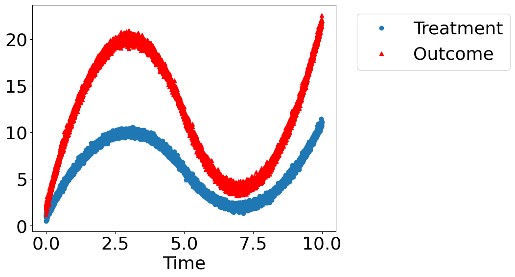
让我们创建一个神秘数据集，我们需要确定是否存在因果效应。

创建数据集。数据集由以下两种模型之一生成：* 模型 1：处理导致结果。* 模型 2：处理不导致结果。所有观测到的相关性均由共同原因引起。

rvar = 1 if np.random.uniform() >0.5 else 0
data_dict = dowhy.datasets.xy_dataset(10000, effect=rvar,
                                      num_common_causes=1,
                                      sd_error=0.2)
df = data_dict['df']
print(df[["Treatment", "Outcome", "w0"]].head())

   Treatment    Outcome        w0
0   7.588773  15.439320  1.483548
1   8.464945  17.079393  2.464048
2   1.985935   4.099270 -3.865950
3   7.118398  13.774239  0.746508
4   3.870168   7.347380 -2.322948

dowhy.plotter.plot_treatment_outcome(df[data_dict["treatment_name"]], df[data_dict["outcome_name"]],
                             df[data_dict["time_val"]])

使用 DoWhy 解决这个谜团：处理是否会导致结果？

步骤 1：将问题建模为因果图

初始化因果模型。

model= CausalModel(
        data=df,
        treatment=data_dict["treatment_name"],
        outcome=data_dict["outcome_name"],
        common_causes=data_dict["common_causes_names"],
        instruments=data_dict["instrument_names"])
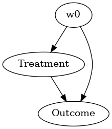
model.view_model(layout="dot")

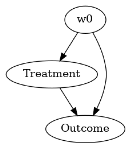
显示存储在本地文件“causal_model.png”中的因果模型

from IPython.display import Image, display
display(Image(filename="causal_model.png"))

步骤 2：使用形式化因果图的属性识别因果效应

使用因果图的属性识别因果效应。

identified_estimand = model.identify_effect(proceed_when_unidentifiable=True)
print(identified_estimand)

Estimand type: EstimandType.NONPARAMETRIC_ATE

### Estimand : 1
Estimand name: backdoor
Estimand expression:
     d
────────────(E[Outcome|w0])
d[Treatment]
Estimand assumption 1, Unconfoundedness: If U→{Treatment} and U→Outcome then P(Outcome|Treatment,w0,U) = P(Outcome|Treatment,w0)

### Estimand : 2
Estimand name: iv
No such variable(s) found!

### Estimand : 3
Estimand name: frontdoor
No such variable(s) found!

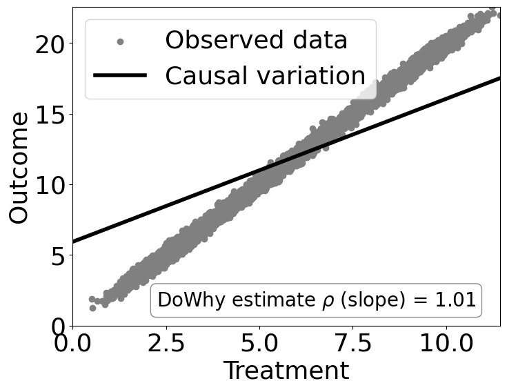
步骤 3：估计因果效应

一旦我们确定了可估计量，就可以使用任何统计方法来估计因果效应。

为了简单起见，我们使用线性回归。

estimate = model.estimate_effect(identified_estimand,
        method_name="backdoor.linear_regression")
print("Causal Estimate is " + str(estimate.value))

# Plot Slope of line between treamtent and outcome =causal effect
dowhy.plotter.plot_causal_effect(estimate, df[data_dict["treatment_name"]], df[data_dict["outcome_name"]])

Causal Estimate is 1.0121551154547133

检查估计是否正确

print("DoWhy estimate is " + str(estimate.value))
print ("Actual true causal effect was {0}".format(rvar))

DoWhy estimate is 1.0121551154547133
Actual true causal effect was 1

步骤 4：反驳估计

我们还可以反驳估计，以检查其对假设的鲁棒性（即敏感性分析，但更强劲）。

添加一个随机共同原因变量

res_random=model.refute_estimate(identified_estimand, estimate, method_name="random_common_cause")
print(res_random)

Refute: Add a random common cause
Estimated effect:1.0121551154547133
New effect:1.0121408959949347
p value:0.96

用随机（安慰剂）变量替换处理

res_placebo=model.refute_estimate(identified_estimand, estimate,
        method_name="placebo_treatment_refuter", placebo_type="permute")
print(res_placebo)

Refute: Use a Placebo Treatment
Estimated effect:1.0121551154547133
New effect:-7.908637019507836e-05
p value:1.0

移除数据的随机子集

res_subset=model.refute_estimate(identified_estimand, estimate,
        method_name="data_subset_refuter", subset_fraction=0.9)
print(res_subset)

Refute: Use a subset of data
Estimated effect:1.0121551154547133
New effect:1.0119332285840539
p value:0.96

如您所见，我们的因果估计器对简单的反驳具有鲁棒性。